Introduction

The heat shock response is a highly conserved mechanism responsible for the maintenance of cellular function under stress. Originally identified as part of the response to increased environmental temperatures (Ritossa 1962) heat shock proteins (HSPs) have since been implicated in susceptibility to infection (Kee et al. 2008), cancer risk (Sfar et al. 2010) and drug response (Martin et al. 2004). Despite its obvious significance many details of the heat shock response still remain uncertain.

Here we study the genome-wide changes to gene expression induced by heat shock in 60 HapMap cell lines from Yoruba individuals (Gibbs 2010) to identify genes and pathways involved in the human heat shock response. To further elucidate underlying mechanisms genetic variants modulating gene expression are mapped across all relevant genes.

Methods

Pre-processing and Quality Control

Raw gene expression QC

rawIntensity <- readr::read_tsv("data/TPS00590_FinalReport_12Oct09.txt", skip = 8, 
    progress = FALSE)

sig.col <- seq(3, 722, 6)
det.col <- seq(8, 722, 6)

sig.data.raw <- rawIntensity[, sig.col]
det.data.raw <- rawIntensity[, det.col]

names(sig.data.raw) <- gsub(":AVG_Signal", "", names(sig.data.raw))
names(det.data.raw) <- gsub(":Detection Pval", "", names(det.data.raw))

info <- readr::read_tsv("data/YRI_sample_list_file_03NOV09.txt", col_types = list(`Date of Harvest` = col_date("%d.%m.%y"), 
    `Date of RNA extraction` = col_date("%d.%m.%y")))

## remove empty lines at end of file
info <- info[1:120, ]
factors <- which(sapply(info, is.factor))
for (i in factors) {
    info[[i]] <- factor(as.character(info[[i]]))
}
info[["Cell Line"]] <- sub("^GM", "NA", info[["Cell Line"]])
info[["Cell Line"]] <- sub("_.$", "", info[["Cell Line"]])
info <- mutate(info, sample = paste(`Cell Line`, Treatment, sep = "_"))

newNames <- paste(info[["Cell Line"]], info$Treatment, sep = "_")
names(newNames) <- info[["ARRAY CODE"]]

## typo in sample ID
names(sig.data.raw)[13] <- "NM-75"
names(det.data.raw)[13] <- "NM-75"

names(sig.data.raw) <- gsub("-", "_", fixed = TRUE, names(sig.data.raw))
names(det.data.raw) <- gsub("-", "_", fixed = TRUE, names(det.data.raw))  #differing name format
names(sig.data.raw) <- newNames[names(sig.data.raw)]
names(det.data.raw) <- newNames[names(det.data.raw)]

sig.data.raw <- cbind(probe = rawIntensity$ProbeID, sig.data.raw)
det.data.raw <- cbind(probe = rawIntensity$ProbeID, det.data.raw)

sig.data.log <- cbind(probe = rawIntensity$ProbeID, log2(sig.data.raw[-1]))

Probe intensities for resting and stimulated cells were imported into R for further processing together with associated meta data.

exclude <- list()
exclude$sample <- character()
exclude$probe <- character()
sig.data.long <- reshapeData(sig.data.log, "intensity")
sig.data.raw.long <- reshapeData(sig.data.raw, "intensity")
det.data.long <- reshapeData(det.data.raw, "p.value")

Annotations for all probes were obtained via the illuminaHumanv3.db Bioconductor package (Barbosa-Morais et al. 2010). Only probes that are considered to be of perfect or good quality were taken forward for analysis. Additionally, all probes mapping to more than one genomic location or to a location that contains a known SNP were excluded.

annot <- illuminaHumanv3fullReannotation()
exclude$probe <- union(exclude$probe, dplyr::filter(annot, !grepl("Good|Perfect", 
    ProbeQuality) | !is.na(OverlappingSNP) | !is.na(RepeatMask))$ArrayAddress)
annot <- dplyr::filter(annot, !ArrayAddress %in% exclude$probe)

txdb <- TxDb.Hsapiens.UCSC.hg19.knownGene
probePos <- strsplit(dplyr::filter(annot, !is.na(GenomicLocation))$GenomicLocation, 
    "[:, ]")
probePos <- data.frame(ArrayAddress = dplyr::filter(annot, !is.na(GenomicLocation))$ArrayAddress, 
    chrom = sapply(probePos, "[[", 1), start = as.numeric(sapply(probePos, "[[", 
        2)), end = as.numeric(sapply(probePos, "[[", 3)), strand = sapply(probePos, 
        "[[", 4))
probePos <- makeGRangesFromDataFrame(probePos, keep.extra.columns = TRUE)
tx <- transcriptsByOverlaps(txdb, probePos)
hits <- findOverlaps(probePos, tx)
probeTx <- data.frame(ArrayAddress = probePos$ArrayAddress[queryHits(hits)], 
    tx_id = tx$tx_id[subjectHits(hits)])
tx2gene <- transcripts(txdb, vals = list(tx_id = unique(probeTx$tx_id)), columns = c("tx_id", 
    "gene_id"))
tx2gene <- dplyr::select(as.data.frame(tx2gene), tx_id, gene_id)
probeGene <- dplyr::left_join(probeTx, tx2gene, by = "tx_id")
probeGene <- unique(dplyr::select(probeGene, ArrayAddress, gene_id))
probeGene$gene_id <- as.character(probeGene$gene_id)

excl <- table(probeGene$ArrayAddress)
exclude$probe <- union(exclude$probe, names(excl)[excl > 1])
annot <- dplyr::filter(annot, !ArrayAddress %in% exclude$probe)

annot <- dplyr::left_join(annot, probeGene, by = "ArrayAddress")
## Warning in left_join_impl(x, y, by$x, by$y): joining factor and character
## vector, coercing into character vector
annot$EntrezReannoated <- ifelse(is.na(annot$gene_id), annot$EntrezReannotated, 
    annot$gene_id)
annot <- dplyr::select(annot, -gene_id)

eg <- mappedkeys(org.Hs.egSYMBOL)
symbols <- as.list(org.Hs.egSYMBOL[eg])
symbols <- data.frame(entrez = names(symbols), symbol = unlist(symbols), stringsAsFactors = FALSE)
annot <- dplyr::left_join(annot, symbols, by = c(EntrezReannotated = "entrez"))
annot$SymbolReannotated <- ifelse(is.na(annot$symbol), annot$SymbolReannotated, 
    annot$symbol)
annot <- dplyr::select(annot, -symbol)
det.pval <- 0.01
det.n <- 10
sample.missing <- 0.7
sd.min <- 0.8

Probes were required to exhibit significant signal (detection p-value < 0.01) in at least 10 samples and samples with less than 30% of the remaining probes providing significant signal were excluded (together with the paired sample). Samples showing exceptionally low variation in probe intensities (standard deviation of the log intensities of all retained probes below 0.8) were also removed.

detected <- tally(group_by(subset(det.data.long, p.value < det.pval), probe))
exclude$probe <- union(exclude$probe, filter(detected, n < det.n)$probe)
sig.data.long <- filter(sig.data.long, !probe %in% exclude$probe)
sig.data.raw.long <- filter(sig.data.raw.long, !probe %in% exclude$probe)
det.data.long <- filter(det.data.long, !probe %in% exclude$probe)
missingSample <- tally(group_by(filter(det.data.long, p.value > det.pval), sample, 
    treatment))
missingSample$n <- missingSample$n/count(det.data.long, sample, treatment)$n
exclude$sample <- union(exclude$sample, filter(missingSample, n >= sample.missing)$sample)
sampleSD <- summarise(group_by(filter(sig.data.long, is.finite(intensity)), 
    sample, treatment), sd(intensity))
exclude$sample <- union(exclude$sample, filter(sampleSD, `sd(intensity)` < sd.min)$sample)
dat <- filterSample(sig.data.long, sig.data.raw.long, det.data.long, exclude$sample)
sig.data.long <- dat$sig
sig.data.raw.long <- dat$sig.raw
det.data.long <- dat$det

After filtering 12416 of 48803 probes (25.4%) and 56 samples remain. See Figure 1 for the distributions of intensities for the remaining probes in each sample.

ggplot(sig.data.long, aes(x = intensity, colour = sample, linetype = treatment)) + 
    geom_density() + theme_bw() + guides(colour = "none")

**Figure 1:** Distribution of probe intensities.

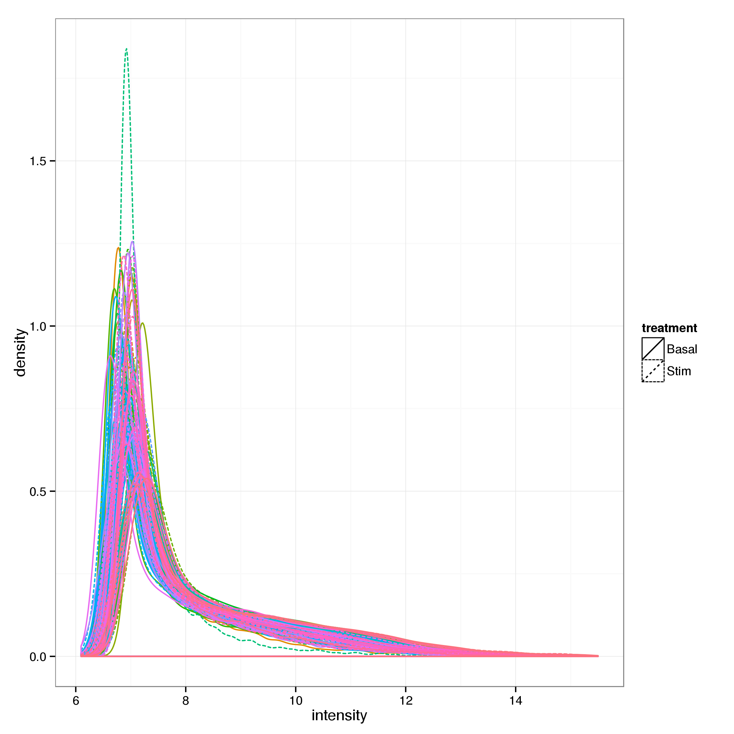
Figure 1: Distribution of probe intensities.

flt <- filter(sig.data.long, !is.finite(intensity))$probe
sig.data.filter <- full_join(spread(filter(sig.data.long, treatment == "Basal" & 
    !probe %in% flt), sample, intensity)[-1], spread(filter(sig.data.long, treatment == 
    "Stim" & !probe %in% flt), sample, intensity)[-1], by = "probe")
names(sig.data.filter) <- sub(".x", "_Basal", names(sig.data.filter), fixed = TRUE)
names(sig.data.filter) <- sub(".y", "_Stim", names(sig.data.filter), fixed = TRUE)

sig.pca <- prcomp(t(sig.data.filter[-1]), scale = TRUE)
sig.pc <- as.data.frame(sig.pca$x)
sig.pc$sample <- rownames(sig.pc)
sig.pc <- dplyr::select(as.tbl(sig.pc), sample, PC1, PC2)
sig.pc <- inner_join(sig.pc, info, by = "sample")

cluster <- dplyr::filter(sig.pc, `Date cRNA Amplified` != "CE_29Sep09")
clusterBound <- chull(cluster$PC1, cluster$PC2)
ggplot(sig.pc, aes(x = PC1, y = PC2)) + geom_polygon(data = cluster[clusterBound, 
    ], fill = "lightgrey", colour = "grey") + geom_point(aes(colour = as.character(Sentrix_ID), 
    shape = `Date cRNA Amplified`), size = 3) + theme_bw() + scale_colour_discrete("BeadChip") + 
    scale_shape_discrete("RNA Amplification")

**Figure 2:** PCA plot of probe intensities by sample. Colours correspond to different BeadChips while shapes indicate different amplification dates. Samples from the two amplifications in October 2009 are clustered together (highlighted by the grey area).

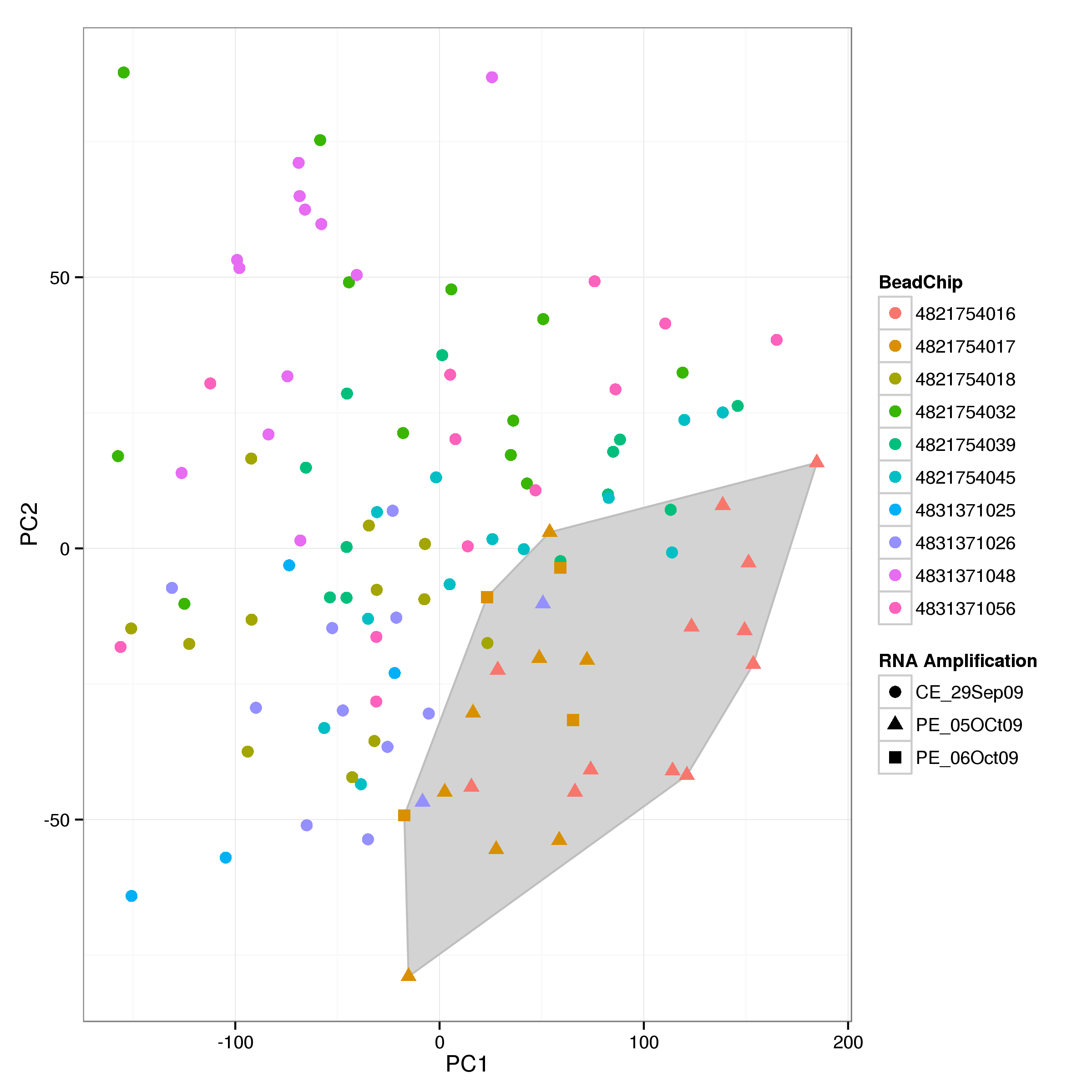
Figure 2: PCA plot of probe intensities by sample. Colours correspond to different BeadChips while shapes indicate different amplification dates. Samples from the two amplifications in October 2009 are clustered together (highlighted by the grey area).

A principle component analysis of the gene expression for the remaining samples indicates a clustering of samples from two RNA amplification batches in October 2009 (Figure 2). This batch effect is noted for later correction during the analysis.

Further analysis of the gene expression response to heat shock revealed that four of the samples (NA18502, NA18508, NA18522, NA18853, NA18504) exhibit patterns of expression inconsistent with those observed in other samples, including reversal of fold change for strongly differentially expressed genes. This suggests a potential mislabelling of these samples, which were consequently excluded.

exclude$sample <- union(exclude$sample, c("NA18502", "NA18508", "NA18522", "NA18853", 
    "NA18504"))
dat <- filterSample(sig.data.long, sig.data.raw.long, det.data.long, exclude$sample)
sig.data.long <- dat$sig
sig.data.raw.long <- dat$sig.raw
det.data.long <- dat$det

Genotype QC

keepSamples <- updateSampleList(sig.data.long$sample, "data/hapmap_YRI_r23a_filtered.fam")
plink --bfile data/hapmap_YRI_r23a_filtered --out tmp/hapmap_yri.snp_flt --keep tmp/sample.lst --maf 0.1 --geno 0.1 --hwe 1e-4 --autosome --make-bed > log/hapmap_yri.snp_flt.log
totalSNPs <- R.utils::countLines("data/hapmap_YRI_r23a_filtered.bim")
remainSNPs <- R.utils::countLines("tmp/hapmap_yri.snp_flt.bim")

Genotype data provided by the HapMap project (Gibbs 2010) was processed with Plink (Chang et al. 2015) to restrict the data to autosomes and remove SNPs with low genotyping rate and and those with a minor allele frequency of less than 10% in the sample. This results in the exclusion of 794511 of 2582999 SNPs (30.76%);

plink --bfile tmp/hapmap_yri.snp_flt --out tmp/hapmap_yri.smpl_flt --mind 0.1 --neighbour 1 3 --genome gz nudge --make-bed > log/hapmap_yri.smpl_flt.log
nnIBS <- readr::read_table("tmp/hapmap_yri.smpl_flt.nearest")

The IBS nearest neighbour calculation shows that the majority of samples are quite similar with regard to the extend of genetic differences between them while a few show markedly increased sharing of alleles (see Figure 3 and Table 1). This is consistent with a population of largely unrelated individuals including a few individuals that are more closely related than expected. One individual (NA18913) also shows evidence of reduced similarity with the second and third nearest neighbour.

ggplot(nnIBS, aes(x = Z, colour = as.factor(NN))) + geom_density(aes(group = NN)) + 
    theme_bw()

**Figure 3:** Similarity between individuals. For each individual the similarity, in terms of IBS, to all other individuals is determined and individuals are ranked acording to this measure. From this a Z-score is computed for for each of the three closest neighbours (see the Plink [documentation](http://pngu.mgh.harvard.edu/~purcell/plink/strat.shtml#outlier) for details). Note the spikes corresponding to individuals with positive Z-scores indicating increased similarity of their genomes compared to the rest of the cohort.

Figure 3: Similarity between individuals. For each individual the similarity, in terms of IBS, to all other individuals is determined and individuals are ranked acording to this measure. From this a Z-score is computed for for each of the three closest neighbours (see the Plink documentation for details). Note the spikes corresponding to individuals with positive Z-scores indicating increased similarity of their genomes compared to the rest of the cohort.

offset <- mean(filter(nnIBS, Z < 0 & NN == 1)$Z)
nnSuspect <- filter(nnIBS, (abs(Z - offset) > 2 & NN == 1) | abs(Z) > 2)
nnSuspect <- nnSuspect[order(abs(nnSuspect$Z), decreasing = TRUE), ]
set.caption(tabRef("nnIBS", "Pairs of Yoruban HapMap samples with evidence of decreased or increased genetic similarity (absolute IBS-based nearest neighbour Z-score > 2)."))
pander(nnSuspect)
Table 1: Pairs of Yoruban HapMap samples with evidence of decreased or increased genetic similarity (absolute IBS-based nearest neighbour Z-score > 2).
FIDIIDNNMIN_DSTZFID2IID2
Yoruba_028NA1891310.81214.343Yoruba_117NA19238
Yoruba_117NA1923810.81214.343Yoruba_028NA18913
Yoruba_024NA1886230.70072.618Yoruba_048NA19203
Yoruba_028NA1891320.6985-2.340Yoruba_048NA19204
Yoruba_028NA1891330.6984-2.325Yoruba_112NA19192
Yoruba_024NA1886220.70092.183Yoruba_017NA18871
Yoruba_101NA1913010.75351.908Yoruba_112NA19192
Yoruba_112NA1919210.75351.908Yoruba_101NA19130
ibdReport <- read.table("tmp/hapmap_yri.smpl_flt.genome.gz", header = TRUE)
ibdSD <- sd(ibdReport$PI_HAT)
ibdHigh <- dplyr::filter(ibdReport, PI_HAT > 2 * ibdSD)

A similar picture emerges if we consider the estimated proportion of IBD for all sample pairs with 3 pairs showing evidence of higher than expected relatedness (see Table 2 and Figure 4 for details).

pairs <- rbind(as.matrix(dplyr::select(ibdHigh, IID1, IID2)), as.matrix(dplyr::select(nnSuspect, 
    IID, IID2)))
exSample <- character()
while (length(pairs)) {
    ids <- sort(table(pairs), decreasing = TRUE)
    exSample <- c(exSample, names(ids[1]))
    pairs <- pairs[!apply(pairs, 1, `%in%`, x = names(ids)[1]), , drop = FALSE]
}
if ("NA19130" %in% exSample && !"NA19192" %in% exSample) {
    exSample[which(exSample == "NA19130")] <- "NA19192"
}

exclude$sample <- union(exclude$sample, exSample)

To ensure that at most one sample of each suspect pair are included in the analysis the samples NA18913, NA19192, NA18862 and NA19092 are excluded.

set.caption(tabRef("ibdHigh", paste("Sample pairs with estimated proportion of IBD exceeding", 
    format(2 * ibdSD, nsmall = 2, digits = 2))))
pander(dplyr::select(ibdHigh, IID1, IID2, PI_HAT, DST, RATIO))
Table 2: Sample pairs with estimated proportion of IBD exceeding 0.032
IID1IID2PI_HATDSTRATIO
NA18913NA192380.50.81276.8
NA19092NA191010.1040.7232.82
NA19130NA191920.2390.7534.5
plot(ibsClust(ibdReport), main = "", xlab = "IBS", sub = "")

**Figure 4:** Dendrogram of individuals included in study. Distances are based on identity by state. Three pairs show clear indications of increased relatedness.

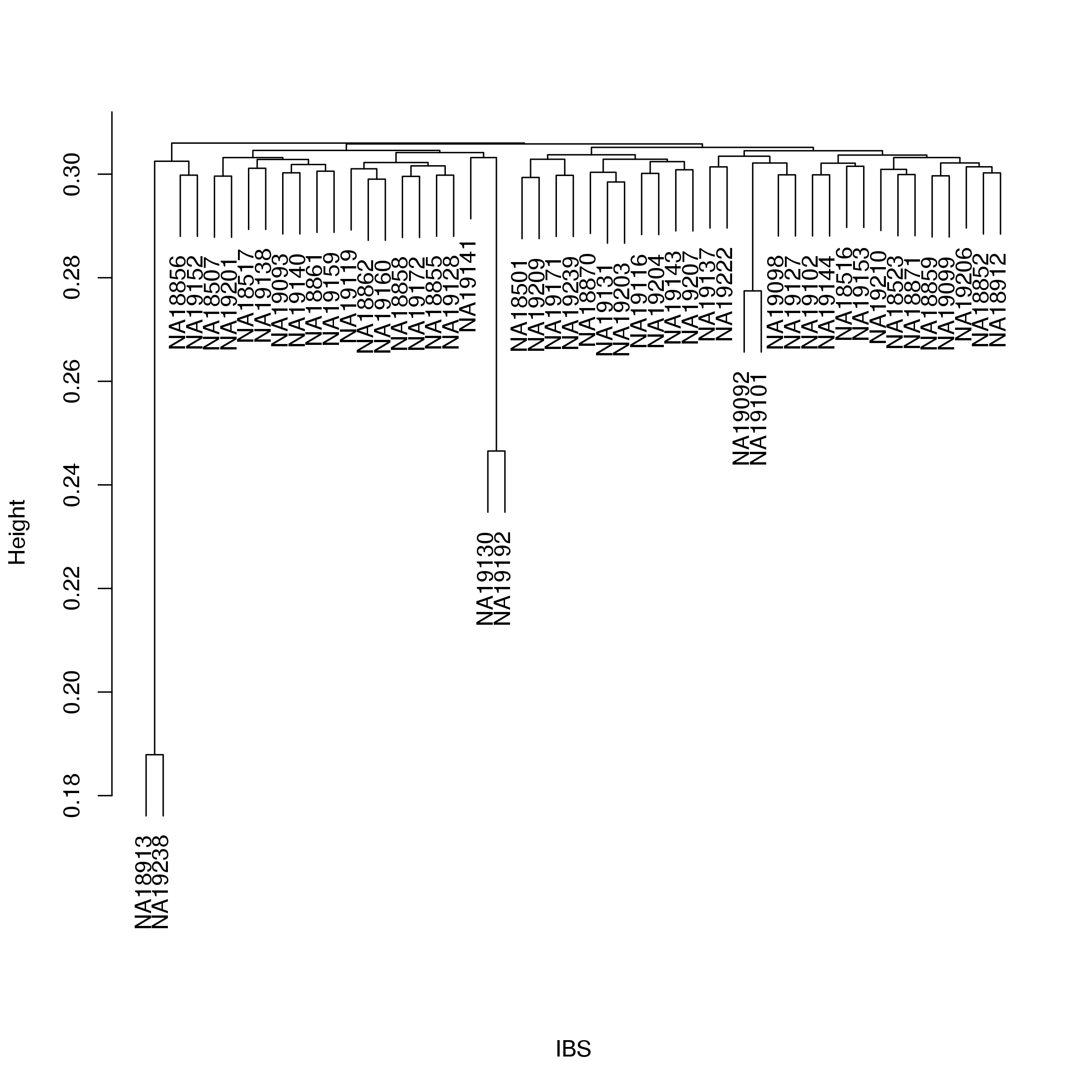
Figure 4: Dendrogram of individuals included in study. Distances are based on identity by state. Three pairs show clear indications of increased relatedness.

dat <- filterSample(sig.data.long, sig.data.raw.long, det.data.long, exclude$sample)
sig.data.long <- dat$sig
sig.data.raw.long <- dat$sig.raw
det.data.long <- dat$det
keepSamples <- updateSampleList(sig.data.long$sample, "data/hapmap_YRI_r23a_filtered.fam")
plink --bfile tmp/hapmap_yri.smpl_flt --out tmp/hapmap_yri.smpl_flt2 --keep tmp/sample.lst --cluster --mds-plot 4 --make-bed > log/hapmap_yri.smpl_flt.log
mds <- read.table("tmp/hapmap_yri.smpl_flt2.mds", header = TRUE)
ggplot(mds, aes(x = C1, y = C2)) + geom_point(size = 3) + theme_bw()

**Figure 5:** MDS plot of samples remaining after genotype QC.

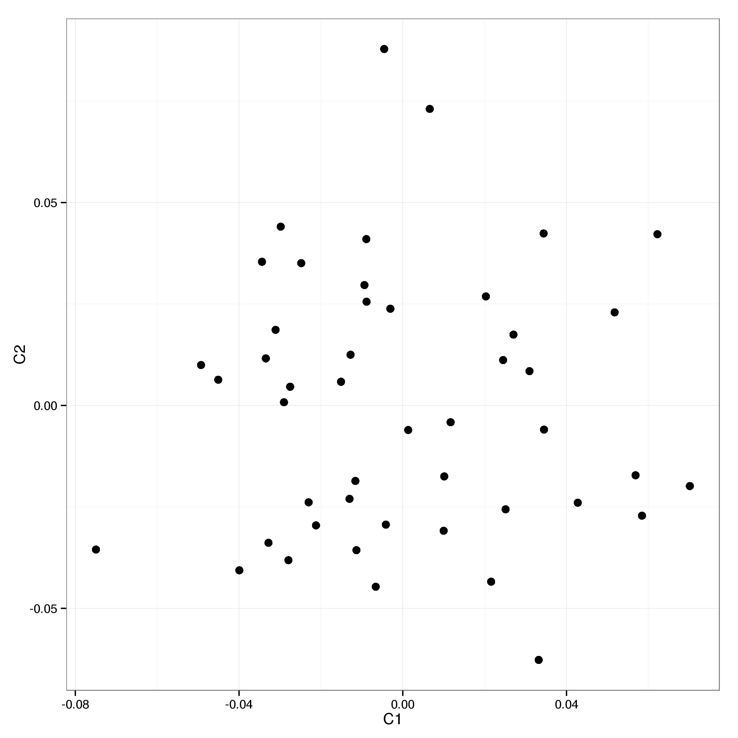
Figure 5: MDS plot of samples remaining after genotype QC.

Plotting the first two MDS components of the remaining 47 samples shows no further evidence for outliers (Figure 5).

Normalising gene expression estimates

sig.data.norm <- justvsn(acast(sig.data.raw.long, formula = probe ~ sample + 
    treatment, value.var = "intensity"))
probeMean <- rowMeans(sig.data.norm)
probeSD <- apply(sig.data.norm, 1, sd)
sig.select <- as.tbl(as.data.frame(sig.data.norm))
sig.select <- mutate(sig.select, mean = probeMean, sd = probeSD)
sig.select <- filter(sig.select, mean > 7)
sig.select <- arrange(sig.select, desc(sd), desc(mean))
sig.select <- head(sig.select, 2000)
sig.pca <- prcomp(t(sig.select), scale = TRUE)
sig.pc <- as.data.frame(sig.pca$x)
sig.pc$sample <- rownames(sig.pc)
sig.pc <- dplyr::select(as.tbl(sig.pc), sample, PC1, PC2, PC3, PC4)
sig.pc <- inner_join(sig.pc, info, by = "sample")
ggOutlier <- outlierPlot(sig.pc, level = 0.985, hjust = 0.2, vjust = -0.5)
sampleCount <- table(ggOutlier$data$Sentrix_ID)
excludeChip <- unique(dplyr::filter(ggOutlier$data, Sentrix_ID %in% names(sampleCount)[sampleCount <= 
    4])$Sentrix_ID)
outlierSample <- unique(dplyr::filter(ggOutlier$data, outlier)$Cell.Line)
chipExclusion <- unique(dplyr::filter(ggOutlier$data, Sentrix_ID %in% excludeChip)$Cell.Line)
exclude$sample <- Reduce(union, list(exclude$sample, outlierSample, chipExclusion))
ggOutlier
## Too few points to calculate an ellipse
## geom_path: Each group consist of only one observation. Do you need to adjust the group aesthetic?

**Figure 6:** PCA plot of normalised gene expression estimates by sample. Each panal is comprised of the remaining samples for a singel BeadChip. For each BeadChip a 99% confidence ellipse is shown. While the majority of samples cluster well within chips some clear ouliers are visible. Variability between chips is relatively high with chips 563403730 and 563403752 appearing distinct from the bulk of the samples.

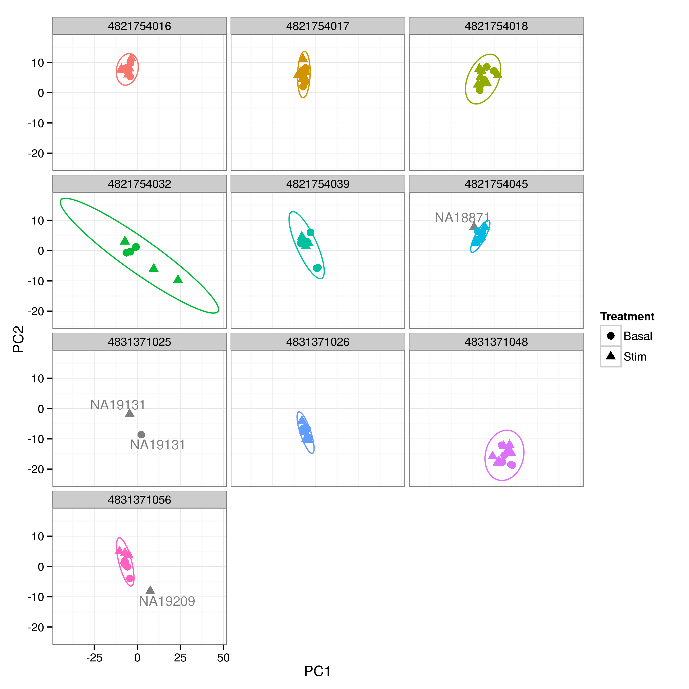
Figure 6: PCA plot of normalised gene expression estimates by sample. Each panal is comprised of the remaining samples for a singel BeadChip. For each BeadChip a 99% confidence ellipse is shown. While the majority of samples cluster well within chips some clear ouliers are visible. Variability between chips is relatively high with chips 563403730 and 563403752 appearing distinct from the bulk of the samples.

Probe intensities were normalised with VSN (Huber et al. 2002). A PCA plot of the initial VSN normalised data (Figure 6) shows clear evidence of samples clustering by BeadChip, as well as 2 obvious outliers, which were removed. In addition the few remaining samples from chip 4831371025 were removed as the entire chip appears to be suspect.

dat <- filterSample(sig.data.long, sig.data.raw.long, det.data.long, exclude$sample)
sig.data.long <- dat$sig
sig.data.raw.long <- dat$sig.raw
det.data.long <- dat$det
keepSamples <- updateSampleList(sig.data.long$sample, "tmp/hapmap_yri.smpl_flt2.fam")
plink --bfile tmp/hapmap_yri.smpl_flt2 --out tmp/hapmap_yri.smpl_flt3 --keep tmp/sample.lst --make-bed > log/hapmap_yri.smpl_flt3.log

The remaining samples were normalised separately for each BeadChip and differences between groups corrected with ComBat (Johnson, Li, and Rabinovic 2007; Leek et al. 2015), preserving differences due to heat shock stimulation.

batch <- with(subset(info, !`Cell Line` %in% exclude$sample), data.frame(sample = sample, 
    cluster = as.integer(factor(Sentrix_ID)), treatment = Treatment, stringsAsFactors = FALSE))
sig.raw <- acast(sig.data.raw.long, formula = probe ~ sample + treatment, value.var = "intensity")
colnames(sig.raw) <- sub("_._", "_", colnames(sig.raw))
sig.raw <- sig.raw[, batch$sample]

vsnFit <- vector(mode = "list", max(batch$cluster))
sig.data.norm <- vector(mode = "list", max(batch$cluster))
for (i in 1:max(batch$cluster)) {
    vsnFit[[i]] <- vsn2(sig.raw[, batch$cluster == i])
    sig.data.norm[[i]] <- predict(vsnFit[[i]], newdata = sig.raw[, batch$cluster == 
        i], useDataInFit = TRUE)
}
sig.data.norm <- do.call(cbind, sig.data.norm)
par(mfrow = c(3, 3))
mapply(meanSdPlot, vsnFit, main = paste("Cluster", 1:max(batch$cluster)), MoreArgs = list(ylim = c(0, 
    1)))

**Figure 7:** VSN fits to grouped dataset.

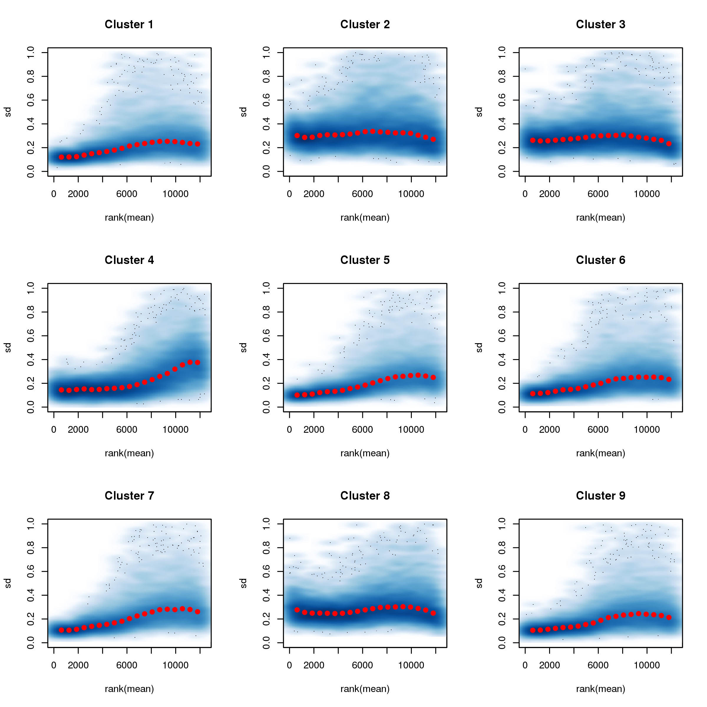
Figure 7: VSN fits to grouped dataset.

par(mfrow = c(1, 1))
batch <- batch[order(batch$cluster), ]
sig.data.norm <- sig.data.norm[, batch$sample]
sig.data.norm <- ComBat(sig.data.norm, batch = batch$cluster, mod = model.matrix(~treatment, 
    data = batch))
## Found 9 batches
## Adjusting for 1 covariate(s) or covariate level(s)
## Standardizing Data across genes
## Fitting L/S model and finding priors
## Finding parametric adjustments
## Adjusting the Data
sig.pca <- prcomp(t(sig.data.norm), scale = TRUE)
sig.pc <- as.data.frame(sig.pca$x)
sig.pc$sample <- rownames(sig.pc)
sig.pc <- dplyr::select(as.tbl(sig.pc), sample, PC1, PC2, PC3, PC4)
sig.pc <- inner_join(sig.pc, info, by = "sample")
ggplot(sig.pc, aes(x = PC1, y = PC2)) + geom_point(aes(colour = as.character(Sentrix_ID)), 
    size = 3) + theme_bw() + scale_colour_discrete("BeadChip")

**Figure 8:** PCA plot of ComBat corrected gene expression.

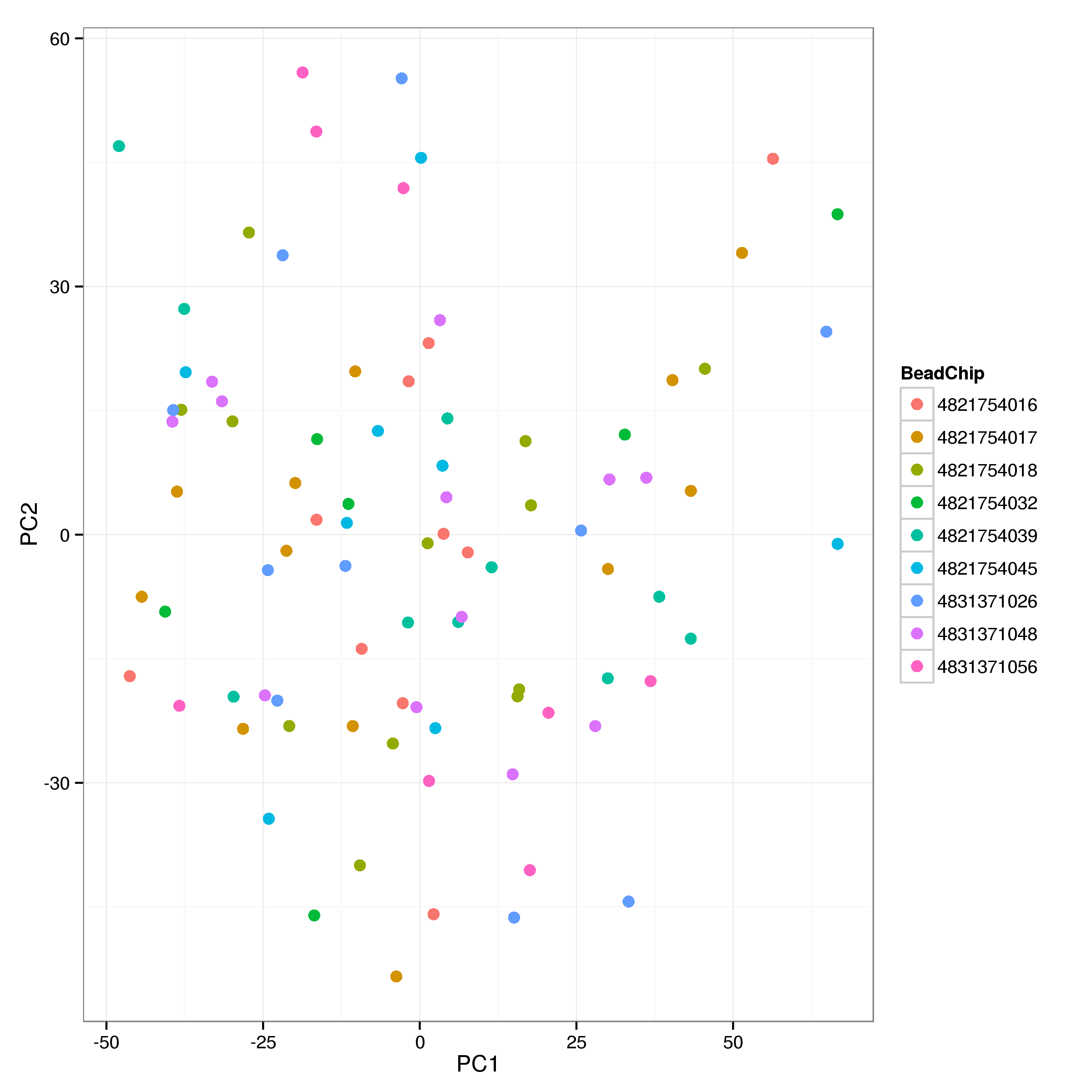
Figure 8: PCA plot of ComBat corrected gene expression.

exprOut <- gzfile("/analysis/tmp/heatshock_expr_norm.tab.gz", open = "w")
write.table(sig.data.norm, file = exprOut, quote = FALSE)
close(exprOut)

Differential expression analysis

All remaining samples were analysed for differences in gene expression between the basal stimulated states, pairing samples from the same individual, using the limma Bioconductor package (M. E. Ritchie et al. 2015).

labels <- strsplit(colnames(sig.data.norm), "_")
sample <- factor(sapply(labels, "[[", 1))
state <- factor(sapply(labels, "[[", 2), levels = c("Basal", "Stim"))
design <- model.matrix(~sample + state)
fit <- lmFit(sig.data.norm, design)
fit <- contrasts.fit(fit, coefficients = "stateStim")
fit <- eBayes(fit)
limmaTable <- topTable(fit, n = length(fit$coefficients))

Individual probes were associated with corresponding genes using the updated annotations provided by the illuminaHumanv3.db Bioconductor package (Barbosa-Morais et al. 2010).

limmaTable <- cbind(ArrayAddress = rownames(limmaTable), limmaTable)
limmaTable <- inner_join(dplyr::select(annot, ArrayAddress, NuID, SymbolReannotated, 
    EntrezReannotated, GenomicLocation), limmaTable)
## Joining by: "ArrayAddress"
## Warning in inner_join_impl(x, y, by$x, by$y): joining character vector and
## factor, coercing into character vector
limmaTable <- limmaTable[order(limmaTable$P.Value), ]
write.table(limmaTable, file = "/analysis/tmp/differential_expression.tab", 
    row.names = FALSE, quote = FALSE, sep = "\t")

Gene N4BP2L2 is associated with two different probes that show evidence of differential expression. One appears to be significantly up regulated while the other is down regulated following heat shock (Table 3). We note that this is the only instance in which multiple probes for a differentially expressed gene provide conflicting evidence in this way. While it is possible that these probes measure two different transcripts that exhibit opposing responses to heat shock we chose to exclude these probes from further analysis to avoid confusion.

set.caption(tabRef("N4BP2L2Table"), "Probes for N4BP2L2")
tab <- dplyr::filter(limmaTable, SymbolReannotated == "N4BP2L2")
tab <- dplyr::select(tab, NuID, SymbolReannotated, logFC, AveExpr, t, P.Value, 
    adj.P.Val, B)
pander(tab)
Quitting from lines 1014-1018 (heatshock_analysis.Rmd)
limmaTable <- dplyr::filter(limmaTable, SymbolReannotated != "N4BP2L2")

GO enrichment analysis

To further investigate the patterns of differential expression a GO enrichment analysis was carried out using the Bioconductor package topGO (Alexa and Rahnenfuhrer 2010). Fisher’s Exact Test was used to determine enrichment separately for significantly (FDR < 0.01) up (Table 4) and down (Table 5) regulated genes.

fdrCut <- 0.01
fcCut <- log2(1.2)

tg <- prep_topGO(limmaTable, fdrCut, fcCut)
## 
## Building most specific GOs ..... ( 8253 GO terms found. )
## 
## Build GO DAG topology .......... ( 11983 GO terms and 28774 relations. )
## 
## Annotating nodes ............... ( 7963 genes annotated to the GO terms. )
## 
## Building most specific GOs ..... ( 8253 GO terms found. )
## 
## Build GO DAG topology .......... ( 11983 GO terms and 28774 relations. )
## 
## Annotating nodes ............... ( 7963 genes annotated to the GO terms. )
## 
## Building most specific GOs ..... ( 8253 GO terms found. )
## 
## Build GO DAG topology .......... ( 11983 GO terms and 28774 relations. )
## 
## Annotating nodes ............... ( 7963 genes annotated to the GO terms. )
resultUp <- runTest(tg$up, algorithm = "classic", statistic = "fisher")
## 
##           -- Classic Algorithm -- 
## 
##       the algorithm is scoring 2722 nontrivial nodes
##       parameters: 
##           test statistic:  fisher
resultDown <- runTest(tg$down, algorithm = "classic", statistic = "fisher")
## 
##           -- Classic Algorithm -- 
## 
##       the algorithm is scoring 2752 nontrivial nodes
##       parameters: 
##           test statistic:  fisher
goTabUp <- GenTable(tg$up, up = resultUp, down = resultDown, topNodes = length(score(resultUp)), 
    orderBy = "up")
goTabUp[["up FDR"]] <- p.adjust(goTabUp$up)
goTabUp[["down FDR"]] <- p.adjust(goTabUp$down)
goTabDown <- GenTable(tg$down, down = resultDown, up = resultUp, topNodes = length(score(resultDown)), 
    orderBy = "down")
goTabDown[["up FDR"]] <- p.adjust(goTabDown$up)
goTabDown[["down FDR"]] <- p.adjust(goTabDown$down)

Gene annotions

In addition to identifying common themes amongst differentially expressed genes the question arises to what extend these genes have been previously associated with the heat shock or, more generally, stress response. We use the set of genes previously linked directly to heat shock (Richter, Haslbeck, and Buchner 2010) and from this create an extended set based on GO terms and PubMed articles linking differentially expressed genes to heat shock response and closely related processes.

knownList <- list()
knownList$known <- readLines("data/heatshock_genes.lst")

Gene Ontology terms

As a first step in highlighting genes not previously known to play a role in this context we identify all significantly up regulated genes that lack GO annotations of obvious relevance to heat shock response. In addition to terms related to stress response and protein folding we also include terms related to cell death and proliferation. To account for the presence of EBV in these cells we ignore all genes annotated with terms related to viral infections. Finally, any remaining genes related to regulation of gene expression are considered to be explained by the large scale changes in gene expression that are taking place in response to heat shock.

sig.entrez <- dplyr::filter(limmaTable, !SymbolReannotated %in% knownList$known, 
    adj.P.Val < fdrCut, logFC > fcCut)$EntrezReannotated
mart <- useMart("ENSEMBL_MART_ENSEMBL", dataset = "hsapiens_gene_ensembl", host = "ensembl.org")
gene.data <- getBM(attributes = c("hgnc_symbol", "entrezgene", "go_id", "name_1006", 
    "namespace_1003"), filters = "entrezgene", values = sig.entrez, mart = mart)
gene.data <- dplyr::filter(gene.data, namespace_1003 == "biological_process")
termFilter_strict <- c("heat", "stress", "folding", "folded")
termFilter_viral <- c("virus", "viral", "immune")
termFilter_extended <- c("death", "apoptosis", "apoptotic", "cell cycle", "mitosis", 
    "mitotic", "proliferation", "transcription", "translation", "gene expression")
termFilter <- c(termFilter_strict, termFilter_extended)

strictGenes <- dplyr::filter(gene.data, str_detect(name_1006, paste(termFilter_strict, 
    collapse = "|")), !str_detect(name_1006, paste(termFilter_viral, collapse = "|")))
extendedGenes <- dplyr::filter(gene.data, str_detect(name_1006, paste(termFilter, 
    collapse = "|")), !str_detect(name_1006, paste(termFilter_viral, collapse = "|")))
knownList$strict <- strictGenes$hgnc_symbol
knownList$extended <- extendedGenes$hgnc_symbol
selGenes_strict <- dplyr::filter(limmaTable, adj.P.Val < fdrCut, logFC > fcCut, 
    !SymbolReannotated %in% knownList$strict, !SymbolReannotated %in% knownList$known)
selGenes <- dplyr::filter(limmaTable, adj.P.Val < fdrCut, logFC > fcCut, !SymbolReannotated %in% 
    knownList$extended, !SymbolReannotated %in% knownList$known)
goKnownList <- knownList
gene.data_all <- getBM(attributes = c("hgnc_symbol", "entrezgene", "go_id", 
    "name_1006", "namespace_1003"), filters = "entrezgene", values = unique(limmaTable$EntrezReannotated), 
    mart = mart)
filterTotal_strict <- dplyr::filter(gene.data_all, str_detect(name_1006, paste(termFilter_strict, 
    collapse = "|")), !str_detect(name_1006, paste(termFilter_viral, collapse = "|")))
filterTotal_extended <- dplyr::filter(gene.data_all, str_detect(name_1006, paste(termFilter, 
    collapse = "|")), !str_detect(name_1006, paste(termFilter_viral, collapse = "|")))
sig.genes <- with(limmaTable, adj.P.Val < fdrCut & logFC > fcCut)
genes_strict <- with(limmaTable, EntrezReannotated %in% filterTotal_strict$entrezgene)
genes_extended <- with(limmaTable, EntrezReannotated %in% filterTotal_extended$entrezgene)
go.test_strict <- fisher.test(sig.genes, genes_strict, alternative = "g")
go.test_extended <- fisher.test(sig.genes, genes_extended, alternative = "g")

PubMed

All genes not annotated with obvious GO terms were subjected to a PubMed search to find publications that link the gene to heat shock or stress response.

selGenes <- dplyr::filter(selGenes, SymbolReannotated != "")
selGenes_strict <- dplyr::filter(selGenes_strict, SymbolReannotated != "")
queryString <- paste(unique(selGenes_strict$SymbolReannotated), "AND (heat shock OR stress)")

query <- vector(mode = "list", length(queryString))
for (i in 1:length(query)) {
    if (i%%10 == 0) 
        Sys.sleep(1)
    query[[i]] <- tryCatch(EUtilsSummary(queryString[i]), error = function(e) {
        Sys.sleep(2)
        EUtilsSummary(queryString[i])
    })
}
names(query) <- unique(selGenes_strict$SymbolReannotated)
queryEmpty <- query[sapply(query, QueryCount) == 0]
queryFound <- query[sapply(query, QueryCount) != 0]


pmids <- vector(mode = "list", length(queryFound))
names(pmids) <- names(queryFound)
for (i in 1:length(pmids)) {
    if (i%%10 == 0) 
        Sys.sleep(1)
    pmids[[i]] <- tryCatch(PMID(EUtilsGet(queryFound[[i]])), error = function(e) {
        Sys.sleep(2)
        PMID(EUtilsGet(queryFound[[i]]))
    })
}
knownList$extended <- union(knownList$extended, names(queryFound))
knownList$strict <- union(knownList$strict, names(queryFound))
knownList$novel <- setdiff(names(queryEmpty), knownList$extended)

putativeGenes <- dplyr::filter(selGenes, SymbolReannotated %in% knownList$novel)
putativeGenes <- dplyr::left_join(putativeGenes, dplyr::select(gene.data, hgnc_symbol, 
    go_id, name_1006), by = c(SymbolReannotated = "hgnc_symbol"))
putativeGenes_strict <- dplyr::filter(selGenes_strict, SymbolReannotated %in% 
    names(queryEmpty))
putativeGenes_strict <- dplyr::left_join(putativeGenes_strict, dplyr::select(gene.data, 
    hgnc_symbol, go_id, name_1006), by = c(SymbolReannotated = "hgnc_symbol"))
write.table(data.frame(gene = names(queryFound), pmid = sapply(pmids, paste, 
    collapse = ",")), file = "tmp/heatshock_pmid.txt", row.names = FALSE, quote = FALSE, 
    sep = "\t")
write.table(putativeGenes, file = "tmp/heatshock_novel.tab", sep = "\t", quote = FALSE, 
    row.names = FALSE)
write.table(putativeGenes_strict, file = "tmp/heatshock_novel_strict.tab", sep = "\t", 
    quote = FALSE, row.names = FALSE)

Heat shock factor binding

To further establish links between differentially expressed genes and heat shock response we consider the evidence for binding of HSF1 and HSF2 in the promoter regions of these genes. Using binding sites derived fro ChIP-seq data obtained from the K562 cell line (Vihervaara et al. 2013) we annotated our list of differentially expressed genes by cross-referencing it with the list HSF binding genes. Groups of genes corresponding to up or down regulated genes as well as those with existing heat shock related annotations and those without were tested for enrichment of HSF binding genes using Fisher’s exact test.

peaks <- list.files(path = "/analysis/data", pattern = "HSF.*\\.txt", full.name = TRUE)

peaks2genes <- data.frame()
for (i in peaks) {
    nm <- gsub("/analysis/data/(.*).txt", "\\1", i)
    f <- read.table(i, sep = "\t", header = T)
    genes <- paste(f[, 11], collapse = ",")
    genes <- unique(strsplit(genes, ",|-")[[1]])
    genes[genes == ""] <- NA
    
    genes <- genes[!is.na(genes)]
    peaks2genes <- rbind(peaks2genes, data.frame(cond = nm, genes = genes))
}
peaks2genes$cond2 <- gsub("^M|^U", "comb", peaks2genes$cond)
peaks2genes$treatment <- str_extract(peaks2genes$cond2, "C|HS")
peaks2genes$tf <- str_extract(peaks2genes$cond2, "HSF.")

peakSplit <- by(peaks2genes, list(peaks2genes$treatment, peaks2genes$tf), function(x) x)
peakSplit[[1]] <- subset(peakSplit[[1]], genes %in% peakSplit[[3]]$genes)
if (nrow(peakSplit[[1]])) {
    peakSplit[[1]]$tf <- "HSF1+HSF2"
    peakSplit[[1]]$cond2 <- paste0(peakSplit[[1]]$cond2, "+HSF2")
}
peakSplit[[2]] <- subset(peakSplit[[2]], genes %in% peakSplit[[4]]$genes)
if (nrow(peakSplit[[2]])) {
    peakSplit[[2]]$tf <- "HSF1+HSF2"
    peakSplit[[2]]$cond2 <- paste0(peakSplit[[2]]$cond2, "+HSF2")
}

peaks2genes <- rbind(peaks2genes, peakSplit[[1]], peakSplit[[2]])
groupUp <- unique(subset(limmaTable, limmaTable$adj.P.Val < fdrCut & limmaTable$logFC > 
    fcCut)$SymbolReannotated)
groupDown <- unique(subset(limmaTable, limmaTable$adj.P.Val < fdrCut & limmaTable$logFC < 
    -fcCut)$SymbolReannotated)

totalNumberOfGenes <- length(unique(limmaTable$SymbolReannotated))
NofgroupUp <- length(groupUp)
NofgroupDown <- length(groupDown)

genes_in_both <- data.frame()
hsfPval <- data.frame()
for (g in unique(peaks2genes$cond2)) {
    anno_genes <- unique(subset(peaks2genes, cond2 == g)$genes)
    groupUp_in_anno_genes <- length(anno_genes[anno_genes %in% groupUp])
    groupUp_not_in_anno_genes <- length(anno_genes[!(anno_genes %in% groupUp)])
    
    groupDown_in_anno_genes <- length(anno_genes[anno_genes %in% groupDown])
    groupDown_not_in_anno_genes <- length(anno_genes[!(anno_genes %in% groupDown)])
    
    if (length(anno_genes[anno_genes %in% groupUp]) > 0) {
        genes_in_both <- rbind(genes_in_both, data.frame(cond = g, exp = "up", 
            genes = anno_genes[anno_genes %in% groupUp]))
    }
    
    if (length(anno_genes[anno_genes %in% groupDown]) > 0) {
        genes_in_both <- rbind(genes_in_both, data.frame(cond = g, exp = "down", 
            genes = anno_genes[anno_genes %in% groupDown]))
    }
    dat_up <- matrix(c(groupUp_in_anno_genes, groupUp_not_in_anno_genes, NofgroupUp, 
        totalNumberOfGenes - NofgroupUp), ncol = 2, byrow = TRUE)
    rst_up <- fisher.test(dat_up, alternative = "greater")
    
    dat_down <- matrix(c(groupDown_in_anno_genes, groupDown_not_in_anno_genes, 
        NofgroupDown, totalNumberOfGenes - NofgroupDown), ncol = 2)
    rst_down <- fisher.test(dat_down, alternative = "greater")
    
    
    hsfPval <- rbind(hsfPval, data.frame(cond = g, up = rst_up$p.value, down = rst_down$p.value, 
        up.or = rst_up$estimate, down.or = rst_down$estimate, sigGenes_up = groupUp_in_anno_genes, 
        sigGenes_down = groupDown_in_anno_genes))
}


genes_in_both$heatshock_novel_genes <- ifelse(genes_in_both$genes %in% knownList$novel, 
    2, ifelse(genes_in_both$genes %in% knownList$extended, 1, 0))

In addition to the direct evidence from the ChIP-seq data we carried out a scan for the presence of HSF binding motifs in the promoter region (1200bp upstream - 300bp downstream of the TSS) of differentially expressed genes. The scan was based on the PWM defined by SwissRegulon (Pachkov et al. 2007) and carried out with the Bioconductor package PWMEnrich (Stojnic and Diez 2014).

txdb <- transcripts(TxDb.Hsapiens.UCSC.hg19.knownGene, columns = c("gene_id", 
    "tx_id", "tx_name"))
promoter.seqs <- getPromoterSeq(txdb, Hsapiens, upstream = 1200, downstream = 300)
names(promoter.seqs) <- as.character(txdb$gene_id)
promoter.seqs <- unique(promoter.seqs)
promoter.seqs_noNA <- promoter.seqs[!is.na(names(promoter.seqs))]

group_up <- dplyr::filter(limmaTable, adj.P.Val < fdrCut, logFC > fcCut)
group_dn <- dplyr::filter(limmaTable, adj.P.Val < fdrCut, logFC < -fcCut)
group_others <- dplyr::filter(limmaTable, !SymbolReannotated %in% group_up$SymbolReannotated, 
    !SymbolReannotated %in% group_dn$SymbolReannotated)

group_up_noNa <- subset(group_up, !is.na(EntrezReannotated))
group_dn_noNa <- subset(group_dn, !is.na(EntrezReannotated))
group_others_noNa <- subset(group_others, !is.na(EntrezReannotated))


promoter.seqs.group_up <- unique(promoter.seqs_noNA[names(promoter.seqs_noNA) %in% 
    group_up_noNa$EntrezReannotated])
promoter.seqs.group_dn <- unique(promoter.seqs_noNA[names(promoter.seqs_noNA) %in% 
    group_dn_noNa$EntrezReannotated])
promoter.seqs.group_others <- unique(promoter.seqs_noNA[names(promoter.seqs_noNA) %in% 
    group_others_noNa$EntrezReannotated])
registerCoresPWMEnrich(4)
motif.HSF1 <- readMotifs("data/HSF1_pwm.jaspar")
genomic.acgt = getBackgroundFrequencies("hg19")
pwms.denovo = toPWM(motif.HSF1, prior = genomic.acgt)
bg.denovo = makeBackground(pwms.denovo, organism = "hg19", type = "logn", quick = TRUE)
## NOTE: Using the 'human' algorithm to infer background parameters,
##       appropriate only for human data.
## Parallel scanning with 4 cores
## Parameter estimation...
## Recording distribution properties for 250 bp tiles (this may take a while...)
## Estimating parameters for motif 1 / 1 
## Recording distribution properties for 500 bp tiles (this may take a while...)
## Estimating parameters for motif 1 / 1 
## Recording distribution properties for 1000 bp tiles (this may take a while...)
## Estimating parameters for motif 1 / 1 
## Recording distribution properties for 2000 bp tiles (this may take a while...)
## Estimating parameters for motif 1 / 1 
## Recording distribution properties for 4000 bp tiles (this may take a while...)
## Estimating parameters for motif 1 / 1

r_promoter.seqs.group_up <- promoterScan(promoter.seqs.group_up, bg.denovo, 
    "up")
## Parallel scanning with 4 cores
## Calculating motif enrichment scores ...
r_promoter.seqs.group_dn <- promoterScan(promoter.seqs.group_dn, bg.denovo, 
    "down")
## Parallel scanning with 4 cores
## Calculating motif enrichment scores ...
r_promoter.seqs.group_others <- promoterScan(promoter.seqs.group_others, bg.denovo, 
    "others")
## Parallel scanning with 4 cores
## Calculating motif enrichment scores ...

r_promoter <- rbind(r_promoter.seqs.group_up, r_promoter.seqs.group_dn, r_promoter.seqs.group_others)
r_promoter <- dplyr::left_join(r_promoter, limmaTable, by = "EntrezReannotated")
## Warning in left_join_impl(x, y, by$x, by$y): joining character vector and
## factor, coercing into character vector
r_promoter$HSFpeak <- ifelse(r_promoter$SymbolReannotated %in% peaks2genes$genes, 
    1, 0)
r_promoter$novel <- ifelse(r_promoter$SymbolReannotated %in% knownList$novel, 
    3, ifelse(r_promoter$SymbolReannotated %in% knownList$extended & !r_promoter$SymbolReannotated %in% 
        knownList$strict, 2, ifelse(r_promoter$SymbolReannotated %in% knownList$strict, 
        1, 0)))

trx_numbers <- data.frame(table(r_promoter$SymbolReannotated))
colnames(trx_numbers) <- c("SymbolReannotated", "trx_numbers")
totalGeneNumber <- nrow(trx_numbers)

genePval <- do.call(rbind, by(r_promoter, r_promoter$SymbolReannotated, function(x) {
    x[which.min(x$p.value), , drop = FALSE]
}))
genePval$pwm.FDR <- p.adjust(genePval$p.value, "BH")
r_promoter <- dplyr::left_join(r_promoter, dplyr::select(genePval, EntrezReannotated, 
    pwm.FDR), by = "EntrezReannotated")
r_promoter <- dplyr::select(r_promoter, -rank, -target, -id)
r_promoter <- dplyr::select(r_promoter, ArrayAddress, NuID, EntrezReannotated, 
    SymbolReannotated, GenomicLocation:B, expr, novel, HSFpeak, raw.score, pwm.p.value = p.value, 
    pwm.FDR)
r_gene <- by(r_promoter, r_promoter$EntrezReannotated, function(x) {
    ans <- x[1, , drop = FALSE]
    if (nrow(x) > 1) {
        exprCols <- c("ArrayAddress", "NuID", "GenomicLocation", "logFC", "AveExpr", 
            "t", "P.Value", "adj.P.Val", "B", "expr")
        pwmCols <- c("raw.score", "pwm.p.value", "pwm.FDR")
        expr <- which.min(x$adj.P.Val)
        ans[1, exprCols] <- x[expr, exprCols]
        pwm <- which.min(x[, "pwm.p.value"])
        ans[1, pwmCols] <- x[pwm, pwmCols]
    }
    ans
})
r_gene <- do.call(rbind, r_gene)
write.table(hsfPval, "tmp/hsf_genes_pvalue.txt", sep = "\t", quote = FALSE, 
    row.names = FALSE)
write.table(genes_in_both, "tmp/hsf_genes.txt", sep = "\t", quote = FALSE, row.names = FALSE)
write.table(r_promoter, "tmp/hsf_motif_genes.txt", sep = "\t", quote = FALSE, 
    row.names = FALSE)
system("tar -czf tmp/gene_annotation.tar.gz -C tmp heatshock_pmid.txt heatshock_novel.tab heatshock_novel_strict.tab hsf_genes.txt hsf_genes_pvalue.txt hsf_motif_genes.txt")

Global heat shock response

To assess the global difference in gene expression induced by heat shock we carried out partial least squares regression (PLS), using the treatment state (basal or stimulated) as a binary response variable and all gene expression probes that passed QC as explanatory variables.

names <- strsplit(colnames(sig.data.norm), "_")
treat <- factor(sapply(names, "[[", 2), levels = c("Basal", "Stim"))
plsFit <- plsreg1(t(sig.data.norm), data.frame(treatment = as.integer(treat) - 
    1))
plsComp <- as.data.frame(plsFit$x.scores)
plsComp$sample <- sapply(names, "[[", 1)
plsComp$treatment <- treat

To explore to what extend this response is modulated by genetic variation we used the length and direction of the response vector, i.e. the vector between the basal and stimulated sample for each individual in the space spanned by the first two PLS components, together with the location of the basal sample in the same space as a multivariate phenotype. This was then tested for association with genotypes for SNPs close to differentially expressed genes and their upstream regulators (identified via Ingenuity Pathway Analysis) using the MultiPhen R package (O’Reilly 2012). The GRCh37 coordinates for SNPs were obtained via the SNPlocs.Hsapiens.dbSNP142.GRCh37 Bioconductor package (Pagès 2014) and gene coordinates via the TxDb.Hsapiens.UCSC.hg19.knownGene package (Carlson 2015).

geno <- read_plink("tmp/hapmap_yri.smpl_flt3")
geno$bim <- dplyr::select(geno$bim, 2, 1, 4)
names(geno$bim) <- c("snp", "chrom", "pos")

geno$bim <- by(geno$bim, geno$bim$chrom, function(x) {
    locs <- getSNPlocs(paste0("ch", x$chrom[1]), caching = FALSE)
    locs$RefSNP_id <- paste0("rs", locs$RefSNP_id)
    snps <- inner_join(x, locs, by = c(snp = "RefSNP_id"))
    if (nrow(snps) < nrow(x)) 
        warning("Dropped ", nrow(x) - nrow(snps), " SNP(s) from chromosome ", 
            x$chrom[1])
    dplyr::select(snps, snp, chrom, loc)
})
## Warning in FUN(data[x, , drop = FALSE], ...): Dropped 243 SNP(s) from
## chromosome 1
## Warning in FUN(data[x, , drop = FALSE], ...): Dropped 251 SNP(s) from
## chromosome 2
## Warning in FUN(data[x, , drop = FALSE], ...): Dropped 159 SNP(s) from
## chromosome 3
## Warning in FUN(data[x, , drop = FALSE], ...): Dropped 154 SNP(s) from
## chromosome 4
## Warning in FUN(data[x, , drop = FALSE], ...): Dropped 141 SNP(s) from
## chromosome 5
## Warning in FUN(data[x, , drop = FALSE], ...): Dropped 1286 SNP(s) from
## chromosome 6
## Warning in FUN(data[x, , drop = FALSE], ...): Dropped 265 SNP(s) from
## chromosome 7
## Warning in FUN(data[x, , drop = FALSE], ...): Dropped 134 SNP(s) from
## chromosome 8
## Warning in FUN(data[x, , drop = FALSE], ...): Dropped 101 SNP(s) from
## chromosome 9
## Warning in FUN(data[x, , drop = FALSE], ...): Dropped 106 SNP(s) from
## chromosome 10
## Warning in FUN(data[x, , drop = FALSE], ...): Dropped 61 SNP(s) from
## chromosome 11
## Warning in FUN(data[x, , drop = FALSE], ...): Dropped 160 SNP(s) from
## chromosome 12
## Warning in FUN(data[x, , drop = FALSE], ...): Dropped 475 SNP(s) from
## chromosome 13
## Warning in FUN(data[x, , drop = FALSE], ...): Dropped 51 SNP(s) from
## chromosome 14
## Warning in FUN(data[x, , drop = FALSE], ...): Dropped 45 SNP(s) from
## chromosome 15
## Warning in FUN(data[x, , drop = FALSE], ...): Dropped 33 SNP(s) from
## chromosome 16
## Warning in FUN(data[x, , drop = FALSE], ...): Dropped 112 SNP(s) from
## chromosome 17
## Warning in FUN(data[x, , drop = FALSE], ...): Dropped 35 SNP(s) from
## chromosome 18
## Warning in FUN(data[x, , drop = FALSE], ...): Dropped 49 SNP(s) from
## chromosome 19
## Warning in FUN(data[x, , drop = FALSE], ...): Dropped 19 SNP(s) from
## chromosome 20
## Warning in FUN(data[x, , drop = FALSE], ...): Dropped 57 SNP(s) from
## chromosome 21
## Warning in FUN(data[x, , drop = FALSE], ...): Dropped 121 SNP(s) from
## chromosome 22

geno$bim <- do.call(rbind, geno$bim)
geno$bim$chrom <- paste0("chr", geno$bim$chrom)
geno$bim <- geno$bim[order(geno$bim$chrom, geno$bim$loc), ]
cisWindow <- 10000

exclChrom <- c("chrX", "chrY", "chrM")
regs <- readr::read_tsv("data/upstream_regulators.tab", progres = FALSE)
regs[[1]] <- stringr::str_extract(regs[[1]], "\\S+")
regs[["FDR"]] <- p.adjust(regs[["P-value"]], method = "BH")
selectedGenes <- dplyr::filter(limmaTable, adj.P.Val < fdrCut & abs(logFC) > 
    fcCut & !str_detect(GenomicLocation, paste(exclChrom, collapse = "|")))
regs <- dplyr::filter(regs, FDR <= 0.01, !`Upstream Regulator` %in% selectedGenes$SymbolReannotated, 
    `Upstream Regulator` %in% limmaTable$SymbolReannotated)
selectedGenes <- rbind(selectedGenes, dplyr::filter(limmaTable, SymbolReannotated %in% 
    regs[["Upstream Regulator"]]))
selectedGenes <- dplyr::select(selectedGenes, ArrayAddress, NuID, GenomicLocation, 
    EntrezReannotated, SymbolReannotated)

selectedGenes$GenomicLocation <- str_extract(selectedGenes$GenomicLocation, 
    "chr[[:digit:]]{1,2}:[[:digit:]]+:[[:digit:]]+")
selectedGenes <- dplyr::filter(selectedGenes, !is.na(GenomicLocation) & !is.na(EntrezReannotated))

txdb <- TxDb.Hsapiens.UCSC.hg19.knownGene
txTable <- select(txdb, keys = selectedGenes$EntrezReannotated, columns = c("TXID", 
    "TXCHROM", "TXSTART", "TXEND"), keytype = "GENEID")
txTable <- dplyr::filter(txTable, !is.na(TXCHROM) & !str_detect(TXCHROM, "_"))
txTable <- by(txTable, txTable$GENEID, function(x) data.frame(entrez = x[["GENEID"]][1], 
    chrom = x[["TXCHROM"]][1], start = min(x[["TXSTART"]]), end = max(x[["TXEND"]])))
txTable <- do.call(rbind, txTable)
selectedGenes <- dplyr::right_join(selectedGenes, txTable, by = c(EntrezReannotated = "entrez"))
## Warning in right_join_impl(x, y, by$x, by$y): joining character vector and
## factor, coercing into character vector

probePos <- dplyr::select(selectedGenes, NuID, chrom, start, end)
probePos <- dplyr::arrange(probePos, chrom, start)

probePosGR <- makeGRangesFromDataFrame(probePos, ignore.strand = TRUE, keep.extra.columns = TRUE)
snpPosGR <- makeGRangesFromDataFrame(geno$bim, ignore.strand = TRUE, keep.extra.columns = TRUE, 
    start.field = "loc", end.field = "loc")
geneSNPs <- do.call(GRangesList, mapply(function(x, chr, s, e) subset(x, seqnames == 
    chr & start >= s - cisWindow & end <= e + cisWindow), as.character(seqnames(probePosGR)), 
    start(probePosGR), end(probePosGR), MoreArgs = list(x = snpPosGR), SIMPLIFY = FALSE))
names(geneSNPs) <- probePos$NuID
noSNP <- probePos$NuID[sapply(geneSNPs, function(x) length(x) == 0)]
snpRange <- unique(unlist(lapply(geneSNPs, function(x) x$snp)))
stimComp <- dplyr::filter(plsComp, treatment == "Stim")
basalComp <- dplyr::filter(plsComp, treatment == "Basal")
globalPheno <- data.frame(sample = stimComp$sample, basal.x = basalComp$t1, 
    basal.y = basalComp$t2, distance = sqrt((stimComp$t1 - basalComp$t1)^2 + 
        (stimComp$t2 - basalComp$t2)^2), direction = atan((stimComp$t2 - basalComp$t2)/(stimComp$t1 - 
        basalComp$t1)))
globalPheno <- dplyr::left_join(globalPheno, dplyr::select(geno$fam, V2, V5), 
    by = c(sample = "V2"))
## Warning in left_join_impl(x, y, by$x, by$y): joining character vector and
## factor, coercing into character vector
globalPheno <- dplyr::rename(globalPheno, sex = V5)

globalPheno <- cbind(scale(dplyr::select(globalPheno, -sex, -sample)), sex = globalPheno$sex - 
    1)
rownames(globalPheno) <- stimComp$sample

rownames(geno$bed) <- str_extract(rownames(geno$bed), "NA[[:digit:]]+$")
cisGeno <- geno$bed[rownames(globalPheno), snpRange]
assoc <- mPhen(cisGeno, globalPheno, covariates = "sex")
## [1] "excluding 0 samples based on exclusion criteria"
idx <- order(assoc$Results[1, , "JointModel", 2])
assoc$Results <- assoc$Results[, idx, , ]
assoc$maf <- assoc$maf[idx]
assoc$adj.p.val <- p.adjust(assoc$Results[, "JointModel", "pvalue"], "BH")

Significance of the observed associations was assessed through a permutation test to account for the structure inherent to the data.

set.seed(54864548L)
nPerm <- 1000
bins <- sapply(apply(cisGeno, 2, table), paste, collapse = "_")
names(bins) <- colnames(cisGeno)
pPerm <- matrix(NA, nrow = nPerm, ncol = length(unique(bins)))
colnames(pPerm) <- unique(bins)
binSNPs <- tapply(colnames(cisGeno), bins, function(x) x)
permGeno <- cisGeno[, sapply(binSNPs, "[", 1)]

for (i in 1:nPerm) {
    permPheno <- dplyr::sample_n(as.data.frame(globalPheno), nrow(globalPheno), 
        replace = FALSE)
    rownames(permPheno) <- rownames(globalPheno)
    assocPerm <- tryCatch(mPhen(permGeno, as.matrix(permPheno), covariates = "sex"), 
        error = function(e) {
            permPheno <- dplyr::sample_n(as.data.frame(globalPheno), nrow(globalPheno), 
                replace = FALSE)
            mPhen(permGeno, as.matrix(permPheno), covariates = "sex")
        })
    pPerm[i, ] <- assocPerm$Results[1, , "JointModel", 2]
}
## Warning: glm.fit: algorithm did not converge
## Warning: glm.fit: fitted probabilities numerically 0 or 1 occurred
## Warning: glm.fit: algorithm did not converge
## Warning: glm.fit: fitted probabilities numerically 0 or 1 occurred

## Warning: glm.fit: fitted probabilities numerically 0 or 1 occurred
## Warning: glm.fit: algorithm did not converge
## Warning: glm.fit: fitted probabilities numerically 0 or 1 occurred

## Warning: glm.fit: fitted probabilities numerically 0 or 1 occurred

## Warning: glm.fit: fitted probabilities numerically 0 or 1 occurred

## Warning: glm.fit: fitted probabilities numerically 0 or 1 occurred

## Warning: glm.fit: fitted probabilities numerically 0 or 1 occurred

## Warning: glm.fit: fitted probabilities numerically 0 or 1 occurred

## Warning: glm.fit: fitted probabilities numerically 0 or 1 occurred
## Warning: glm.fit: algorithm did not converge
## Warning: glm.fit: fitted probabilities numerically 0 or 1 occurred
## Warning: glm.fit: algorithm did not converge
## Warning: glm.fit: fitted probabilities numerically 0 or 1 occurred
## Warning: glm.fit: algorithm did not converge
## Warning: glm.fit: fitted probabilities numerically 0 or 1 occurred
## Warning: glm.fit: algorithm did not converge
## Warning: glm.fit: fitted probabilities numerically 0 or 1 occurred

## Warning: glm.fit: fitted probabilities numerically 0 or 1 occurred

## Warning: glm.fit: fitted probabilities numerically 0 or 1 occurred

## Warning: glm.fit: fitted probabilities numerically 0 or 1 occurred

## Warning: glm.fit: fitted probabilities numerically 0 or 1 occurred

## Warning: glm.fit: fitted probabilities numerically 0 or 1 occurred

## Warning: glm.fit: fitted probabilities numerically 0 or 1 occurred

## Warning: glm.fit: fitted probabilities numerically 0 or 1 occurred

## Warning: glm.fit: fitted probabilities numerically 0 or 1 occurred

## Warning: glm.fit: fitted probabilities numerically 0 or 1 occurred

## Warning: glm.fit: fitted probabilities numerically 0 or 1 occurred

## Warning: glm.fit: fitted probabilities numerically 0 or 1 occurred
## Warning: glm.fit: algorithm did not converge
## Warning: glm.fit: fitted probabilities numerically 0 or 1 occurred

## Warning: glm.fit: fitted probabilities numerically 0 or 1 occurred

## Warning: glm.fit: fitted probabilities numerically 0 or 1 occurred

## Warning: glm.fit: fitted probabilities numerically 0 or 1 occurred

## Warning: glm.fit: fitted probabilities numerically 0 or 1 occurred

## Warning: glm.fit: fitted probabilities numerically 0 or 1 occurred

## Warning: glm.fit: fitted probabilities numerically 0 or 1 occurred

## Warning: glm.fit: fitted probabilities numerically 0 or 1 occurred

## Warning: glm.fit: fitted probabilities numerically 0 or 1 occurred

## Warning: glm.fit: fitted probabilities numerically 0 or 1 occurred

## Warning: glm.fit: fitted probabilities numerically 0 or 1 occurred

## Warning: glm.fit: fitted probabilities numerically 0 or 1 occurred

## Warning: glm.fit: fitted probabilities numerically 0 or 1 occurred

## Warning: glm.fit: fitted probabilities numerically 0 or 1 occurred

## Warning: glm.fit: fitted probabilities numerically 0 or 1 occurred

## Warning: glm.fit: fitted probabilities numerically 0 or 1 occurred

## Warning: glm.fit: fitted probabilities numerically 0 or 1 occurred

## Warning: glm.fit: fitted probabilities numerically 0 or 1 occurred

## Warning: glm.fit: fitted probabilities numerically 0 or 1 occurred

## Warning: glm.fit: fitted probabilities numerically 0 or 1 occurred

## Warning: glm.fit: fitted probabilities numerically 0 or 1 occurred

## Warning: glm.fit: fitted probabilities numerically 0 or 1 occurred
## Warning: glm.fit: algorithm did not converge
## Warning: glm.fit: fitted probabilities numerically 0 or 1 occurred

## Warning: glm.fit: fitted probabilities numerically 0 or 1 occurred

## Warning: glm.fit: fitted probabilities numerically 0 or 1 occurred

## Warning: glm.fit: fitted probabilities numerically 0 or 1 occurred

## Warning: glm.fit: fitted probabilities numerically 0 or 1 occurred

## Warning: glm.fit: fitted probabilities numerically 0 or 1 occurred

## Warning: glm.fit: fitted probabilities numerically 0 or 1 occurred

## Warning: glm.fit: fitted probabilities numerically 0 or 1 occurred

## Warning: glm.fit: fitted probabilities numerically 0 or 1 occurred

## Warning: glm.fit: fitted probabilities numerically 0 or 1 occurred

## Warning: glm.fit: fitted probabilities numerically 0 or 1 occurred
## Warning: glm.fit: algorithm did not converge
## Warning: glm.fit: fitted probabilities numerically 0 or 1 occurred

## Warning: glm.fit: fitted probabilities numerically 0 or 1 occurred

## Warning: glm.fit: fitted probabilities numerically 0 or 1 occurred

## Warning: glm.fit: fitted probabilities numerically 0 or 1 occurred

## Warning: glm.fit: fitted probabilities numerically 0 or 1 occurred

## Warning: glm.fit: fitted probabilities numerically 0 or 1 occurred

## Warning: glm.fit: fitted probabilities numerically 0 or 1 occurred

## Warning: glm.fit: fitted probabilities numerically 0 or 1 occurred

## Warning: glm.fit: fitted probabilities numerically 0 or 1 occurred
## Warning: glm.fit: algorithm did not converge
## Warning: glm.fit: fitted probabilities numerically 0 or 1 occurred

## Warning: glm.fit: fitted probabilities numerically 0 or 1 occurred

## Warning: glm.fit: fitted probabilities numerically 0 or 1 occurred
## Warning: glm.fit: algorithm did not converge
## Warning: glm.fit: fitted probabilities numerically 0 or 1 occurred

## Warning: glm.fit: fitted probabilities numerically 0 or 1 occurred

## Warning: glm.fit: fitted probabilities numerically 0 or 1 occurred
## Warning: glm.fit: algorithm did not converge
## Warning: glm.fit: fitted probabilities numerically 0 or 1 occurred

## Warning: glm.fit: fitted probabilities numerically 0 or 1 occurred

## Warning: glm.fit: fitted probabilities numerically 0 or 1 occurred

## Warning: glm.fit: fitted probabilities numerically 0 or 1 occurred

## Warning: glm.fit: fitted probabilities numerically 0 or 1 occurred

## Warning: glm.fit: fitted probabilities numerically 0 or 1 occurred

## Warning: glm.fit: fitted probabilities numerically 0 or 1 occurred

## Warning: glm.fit: fitted probabilities numerically 0 or 1 occurred

## Warning: glm.fit: fitted probabilities numerically 0 or 1 occurred

## Warning: glm.fit: fitted probabilities numerically 0 or 1 occurred
## Warning: glm.fit: algorithm did not converge
## Warning: glm.fit: fitted probabilities numerically 0 or 1 occurred

## Warning: glm.fit: fitted probabilities numerically 0 or 1 occurred

## Warning: glm.fit: fitted probabilities numerically 0 or 1 occurred

## Warning: glm.fit: fitted probabilities numerically 0 or 1 occurred
## Warning: glm.fit: algorithm did not converge
## Warning: glm.fit: fitted probabilities numerically 0 or 1 occurred

## Warning: glm.fit: fitted probabilities numerically 0 or 1 occurred
## Warning: glm.fit: algorithm did not converge
## Warning: glm.fit: fitted probabilities numerically 0 or 1 occurred
## Warning: glm.fit: algorithm did not converge
## Warning: glm.fit: fitted probabilities numerically 0 or 1 occurred

## Warning: glm.fit: fitted probabilities numerically 0 or 1 occurred

## Warning: glm.fit: fitted probabilities numerically 0 or 1 occurred

## Warning: glm.fit: fitted probabilities numerically 0 or 1 occurred

## Warning: glm.fit: fitted probabilities numerically 0 or 1 occurred

## Warning: glm.fit: fitted probabilities numerically 0 or 1 occurred

## Warning: glm.fit: fitted probabilities numerically 0 or 1 occurred

## Warning: glm.fit: fitted probabilities numerically 0 or 1 occurred

## Warning: glm.fit: fitted probabilities numerically 0 or 1 occurred

## Warning: glm.fit: fitted probabilities numerically 0 or 1 occurred

## Warning: glm.fit: fitted probabilities numerically 0 or 1 occurred
## Warning: glm.fit: algorithm did not converge
## Warning: glm.fit: fitted probabilities numerically 0 or 1 occurred
## Warning: glm.fit: algorithm did not converge
## Warning: glm.fit: fitted probabilities numerically 0 or 1 occurred

## Warning: glm.fit: fitted probabilities numerically 0 or 1 occurred

## Warning: glm.fit: fitted probabilities numerically 0 or 1 occurred

## Warning: glm.fit: fitted probabilities numerically 0 or 1 occurred

## Warning: glm.fit: fitted probabilities numerically 0 or 1 occurred

## Warning: glm.fit: fitted probabilities numerically 0 or 1 occurred

## Warning: glm.fit: fitted probabilities numerically 0 or 1 occurred

## Warning: glm.fit: fitted probabilities numerically 0 or 1 occurred

## Warning: glm.fit: fitted probabilities numerically 0 or 1 occurred

## Warning: glm.fit: fitted probabilities numerically 0 or 1 occurred
## Warning: glm.fit: algorithm did not converge
## Warning: glm.fit: fitted probabilities numerically 0 or 1 occurred
## Warning: glm.fit: algorithm did not converge
## Warning: glm.fit: fitted probabilities numerically 0 or 1 occurred
## Warning: glm.fit: algorithm did not converge
## Warning: glm.fit: fitted probabilities numerically 0 or 1 occurred

## Warning: glm.fit: fitted probabilities numerically 0 or 1 occurred
## Warning: glm.fit: algorithm did not converge
## Warning: glm.fit: fitted probabilities numerically 0 or 1 occurred
## Warning: glm.fit: algorithm did not converge
## Warning: glm.fit: fitted probabilities numerically 0 or 1 occurred

## Warning: glm.fit: fitted probabilities numerically 0 or 1 occurred

## Warning: glm.fit: fitted probabilities numerically 0 or 1 occurred

## Warning: glm.fit: fitted probabilities numerically 0 or 1 occurred

## Warning: glm.fit: fitted probabilities numerically 0 or 1 occurred

## Warning: glm.fit: fitted probabilities numerically 0 or 1 occurred
## Warning: glm.fit: algorithm did not converge
## Warning: glm.fit: fitted probabilities numerically 0 or 1 occurred

## Warning: glm.fit: fitted probabilities numerically 0 or 1 occurred

## Warning: glm.fit: fitted probabilities numerically 0 or 1 occurred
## Warning: glm.fit: algorithm did not converge
## Warning: glm.fit: fitted probabilities numerically 0 or 1 occurred
## Warning: glm.fit: algorithm did not converge
## Warning: glm.fit: fitted probabilities numerically 0 or 1 occurred
## Warning: glm.fit: algorithm did not converge
## Warning: glm.fit: fitted probabilities numerically 0 or 1 occurred

## Warning: glm.fit: fitted probabilities numerically 0 or 1 occurred

## Warning: glm.fit: fitted probabilities numerically 0 or 1 occurred

## Warning: glm.fit: fitted probabilities numerically 0 or 1 occurred

## Warning: glm.fit: fitted probabilities numerically 0 or 1 occurred

## Warning: glm.fit: fitted probabilities numerically 0 or 1 occurred

## Warning: glm.fit: fitted probabilities numerically 0 or 1 occurred

## Warning: glm.fit: fitted probabilities numerically 0 or 1 occurred

## Warning: glm.fit: fitted probabilities numerically 0 or 1 occurred

## Warning: glm.fit: fitted probabilities numerically 0 or 1 occurred

## Warning: glm.fit: fitted probabilities numerically 0 or 1 occurred

## Warning: glm.fit: fitted probabilities numerically 0 or 1 occurred

## Warning: glm.fit: fitted probabilities numerically 0 or 1 occurred

## Warning: glm.fit: fitted probabilities numerically 0 or 1 occurred

## Warning: glm.fit: fitted probabilities numerically 0 or 1 occurred

## Warning: glm.fit: fitted probabilities numerically 0 or 1 occurred

## Warning: glm.fit: fitted probabilities numerically 0 or 1 occurred
## Warning: glm.fit: algorithm did not converge
## Warning: glm.fit: fitted probabilities numerically 0 or 1 occurred

## Warning: glm.fit: fitted probabilities numerically 0 or 1 occurred

## Warning: glm.fit: fitted probabilities numerically 0 or 1 occurred

## Warning: glm.fit: fitted probabilities numerically 0 or 1 occurred

## Warning: glm.fit: fitted probabilities numerically 0 or 1 occurred
## Warning: glm.fit: algorithm did not converge
## Warning: glm.fit: fitted probabilities numerically 0 or 1 occurred

## Warning: glm.fit: fitted probabilities numerically 0 or 1 occurred
## Warning: glm.fit: algorithm did not converge
## Warning: glm.fit: fitted probabilities numerically 0 or 1 occurred
## Warning: glm.fit: algorithm did not converge
## Warning: glm.fit: fitted probabilities numerically 0 or 1 occurred

## Warning: glm.fit: fitted probabilities numerically 0 or 1 occurred

## Warning: glm.fit: fitted probabilities numerically 0 or 1 occurred

## Warning: glm.fit: fitted probabilities numerically 0 or 1 occurred

## Warning: glm.fit: fitted probabilities numerically 0 or 1 occurred

## Warning: glm.fit: fitted probabilities numerically 0 or 1 occurred

## Warning: glm.fit: fitted probabilities numerically 0 or 1 occurred
## Warning: glm.fit: algorithm did not converge
## Warning: glm.fit: fitted probabilities numerically 0 or 1 occurred
## Warning: glm.fit: algorithm did not converge
## Warning: glm.fit: fitted probabilities numerically 0 or 1 occurred
## Warning: glm.fit: algorithm did not converge
## Warning: glm.fit: fitted probabilities numerically 0 or 1 occurred
## Warning: glm.fit: algorithm did not converge
## Warning: glm.fit: fitted probabilities numerically 0 or 1 occurred

## Warning: glm.fit: fitted probabilities numerically 0 or 1 occurred

## Warning: glm.fit: fitted probabilities numerically 0 or 1 occurred

## Warning: glm.fit: fitted probabilities numerically 0 or 1 occurred

## Warning: glm.fit: fitted probabilities numerically 0 or 1 occurred

## Warning: glm.fit: fitted probabilities numerically 0 or 1 occurred

## Warning: glm.fit: fitted probabilities numerically 0 or 1 occurred

## Warning: glm.fit: fitted probabilities numerically 0 or 1 occurred

## Warning: glm.fit: fitted probabilities numerically 0 or 1 occurred

## Warning: glm.fit: fitted probabilities numerically 0 or 1 occurred

## Warning: glm.fit: fitted probabilities numerically 0 or 1 occurred

## Warning: glm.fit: fitted probabilities numerically 0 or 1 occurred
## Warning: glm.fit: algorithm did not converge
## Warning: glm.fit: fitted probabilities numerically 0 or 1 occurred

## Warning: glm.fit: fitted probabilities numerically 0 or 1 occurred

## Warning: glm.fit: fitted probabilities numerically 0 or 1 occurred

## Warning: glm.fit: fitted probabilities numerically 0 or 1 occurred
## Warning: glm.fit: algorithm did not converge
## Warning: glm.fit: fitted probabilities numerically 0 or 1 occurred

## Warning: glm.fit: fitted probabilities numerically 0 or 1 occurred

## Warning: glm.fit: fitted probabilities numerically 0 or 1 occurred
## Warning: glm.fit: algorithm did not converge
## Warning: glm.fit: fitted probabilities numerically 0 or 1 occurred

## Warning: glm.fit: fitted probabilities numerically 0 or 1 occurred

## Warning: glm.fit: fitted probabilities numerically 0 or 1 occurred
## Warning: glm.fit: algorithm did not converge
## Warning: glm.fit: fitted probabilities numerically 0 or 1 occurred

## Warning: glm.fit: fitted probabilities numerically 0 or 1 occurred

## Warning: glm.fit: fitted probabilities numerically 0 or 1 occurred

## Warning: glm.fit: fitted probabilities numerically 0 or 1 occurred

## Warning: glm.fit: fitted probabilities numerically 0 or 1 occurred
## Warning: glm.fit: algorithm did not converge
## Warning: glm.fit: fitted probabilities numerically 0 or 1 occurred
## Warning: glm.fit: algorithm did not converge
## Warning: glm.fit: fitted probabilities numerically 0 or 1 occurred

## Warning: glm.fit: fitted probabilities numerically 0 or 1 occurred

## Warning: glm.fit: fitted probabilities numerically 0 or 1 occurred

## Warning: glm.fit: fitted probabilities numerically 0 or 1 occurred

## Warning: glm.fit: fitted probabilities numerically 0 or 1 occurred

## Warning: glm.fit: fitted probabilities numerically 0 or 1 occurred

## Warning: glm.fit: fitted probabilities numerically 0 or 1 occurred

## Warning: glm.fit: fitted probabilities numerically 0 or 1 occurred

## Warning: glm.fit: fitted probabilities numerically 0 or 1 occurred

## Warning: glm.fit: fitted probabilities numerically 0 or 1 occurred

## Warning: glm.fit: fitted probabilities numerically 0 or 1 occurred

## Warning: glm.fit: fitted probabilities numerically 0 or 1 occurred

## Warning: glm.fit: fitted probabilities numerically 0 or 1 occurred
## Warning: glm.fit: algorithm did not converge
## Warning: glm.fit: fitted probabilities numerically 0 or 1 occurred

## Warning: glm.fit: fitted probabilities numerically 0 or 1 occurred

## Warning: glm.fit: fitted probabilities numerically 0 or 1 occurred

## Warning: glm.fit: fitted probabilities numerically 0 or 1 occurred

## Warning: glm.fit: fitted probabilities numerically 0 or 1 occurred

## Warning: glm.fit: fitted probabilities numerically 0 or 1 occurred

## Warning: glm.fit: fitted probabilities numerically 0 or 1 occurred

## Warning: glm.fit: fitted probabilities numerically 0 or 1 occurred
## Warning: glm.fit: algorithm did not converge
## Warning: glm.fit: fitted probabilities numerically 0 or 1 occurred

## Warning: glm.fit: fitted probabilities numerically 0 or 1 occurred

## Warning: glm.fit: fitted probabilities numerically 0 or 1 occurred
## Warning: glm.fit: algorithm did not converge
## Warning: glm.fit: fitted probabilities numerically 0 or 1 occurred
## Warning: glm.fit: algorithm did not converge
## Warning: glm.fit: fitted probabilities numerically 0 or 1 occurred

## Warning: glm.fit: fitted probabilities numerically 0 or 1 occurred

## Warning: glm.fit: fitted probabilities numerically 0 or 1 occurred

## Warning: glm.fit: fitted probabilities numerically 0 or 1 occurred
## Warning: glm.fit: algorithm did not converge
## Warning: glm.fit: fitted probabilities numerically 0 or 1 occurred

To this end the observed global response phenotype for each individual and covariates used in the model were randomly assigned to one of the observed set of genotypes 1000 times and p-values for the joint model were computed for each permutation. From these we computed false discovery rates by comparing observed p-values to the empirical distribution of minimum p-values from each permutation.

minp <- apply(pPerm, 1, min)
assoc$adj.p.val <- sapply(assoc$Results[, "JointModel", 2], function(x) sum(minp < 
    x)/length(minp))
names(assoc$adj.p.val) <- dimnames(assoc$Results)[[1]]
assoc$perm.p.val <- numeric(length(assoc$maf))
names(assoc$perm.p.val) <- dimnames(assoc$Results)[[1]]
for (i in 1:ncol(pPerm)) {
    assoc$perm.p.val[binSNPs[[i]]] <- sapply(assoc$Results[binSNPs[[i]], "JointModel", 
        2], function(x, p) sum(p < x)/length(p), pPerm[, i])
}

Following up on the observed associations between SNPs and the global heat shock response we investigated possible associations between these SNPs and differentially expreressed genes implicated in the heat shock response. Here we define the gene set of interest as those genes that were significantly up regulated (FDR < 0.01 and fold change > 1.2) following heat shock and that were found to have HSF1 or HSF2 ChIP-seq peaks or binding motifs (P < 0.05) in their promoter region.

selSymbol <- dplyr::filter(r_gene, expr == "up", HSFpeak == 1 | pwm.p.value < 
    0.05)$SymbolReannotated
selSymbol <- union(selSymbol, c("CDKN1A", regs[["Upstream Regulator"]]))
selectedGenes <- dplyr::filter(limmaTable, SymbolReannotated %in% selSymbol)
probePos <- t(sapply(selectedGenes$GenomicLocation, str_extract, c("^chr([[:digit:]]+|X)(_[[:alnum:]]+_hap[[:digit:]]+)*", 
    ":[[:digit:]]+", "[[:digit:]]+:[+-]")))
rownames(probePos) <- selectedGenes$NuID
probePos[, 2] <- str_replace(probePos[, 2], ":", "")
probePos[, 3] <- str_replace_all(probePos[, 3], "[:+-]", "")
probePos <- cbind(rownames(probePos), probePos)
selectedExpr <- sig.data.norm[selectedGenes$ArrayAddress, ]
basalIdx <- grep("_Basal", colnames(selectedExpr))
stimIdx <- grep("_Stim", colnames(selectedExpr))
selectedFC <- selectedExpr[, stimIdx] - selectedExpr[, basalIdx]
colnames(selectedFC) <- str_extract(colnames(selectedFC), "NA[[:digit:]]+")
rownames(selectedFC) <- selectedGenes$NuID
write.table(selectedFC, file = "tmp/selected_probes_fc.tab", sep = "\t", quote = FALSE)
rownames(geno$bed) <- str_extract(rownames(geno$bed), "NA[[:digit:]]+")
geno$bed <- geno$bed[colnames(selectedFC), geno$bim$snp]
geno$bed <- t(geno$bed)
flip <- rowSums(geno$bed, na.rm = TRUE) > ncol(geno$bed)
if (any(flip)) {
    geno$bed[flip, ] <- -geno$bed[flip] + 2
}
selGlobal <- dimnames(assoc$Result)[[1]][which(assoc$adj.p.val < 0.1)]
globalSNPs <- geno$bed[selGlobal[c(1, 3)], , drop = FALSE]
write.table(globalSNPs, file = "tmp/global_geno.tab", sep = "\t", quote = FALSE)
stimExpr <- selectedExpr[, stimIdx]
basalExpr <- selectedExpr[, basalIdx]
colnames(stimExpr) <- str_extract(colnames(stimExpr), "NA[[:digit:]]+")
colnames(basalExpr) <- str_extract(colnames(basalExpr), "NA[[:digit:]]+")
rownames(stimExpr) <- rownames(basalExpr) <- selectedGenes$NuID
write.table(stimExpr, file = "tmp/selected_probes_stim_expr.tab", sep = "\t", 
    quote = FALSE)
write.table(basalExpr, file = "tmp/selected_probes_basal_expr.tab", sep = "\t", 
    quote = FALSE)
nPC <- 1
if (nPC > 0) {
    pca <- prcomp(t(selectedFC), center = TRUE, scale = TRUE)
    pc <- pca$x
}
geno$fam <- dplyr::filter(dplyr::select(geno$fam, 2, 5), V2 %in% colnames(geno$bed))
geno$fam <- t(geno$fam)
colnames(geno$fam) <- geno$fam[1, ]
geno$fam <- geno$fam[, colnames(selectedFC)]
covarFC <- geno$fam[-1, , drop = FALSE]
if (nPC > 0) covarFC <- rbind(covarFC, t(pc[, 1:nPC]))
nPC_expr <- 2
if (nPC_expr > 0) {
    pca_stim <- prcomp(t(stimExpr), center = TRUE, scale = TRUE)
    pc_stim <- pca_stim$x
}
covarStim <- geno$fam[-1, , drop = FALSE]
if (nPC_expr > 0) covarStim <- rbind(covarStim, t(pc_stim[, 1:nPC_expr]))

if (nPC_expr > 0) {
    pca_basal <- prcomp(t(basalExpr), center = TRUE, scale = TRUE)
    pc_basal <- pca_basal$x
}
covarBasal <- geno$fam[-1, , drop = FALSE]
if (nPC_expr > 0) covarBasal <- rbind(covarBasal, t(pc_basal[, 1:nPC_expr]))
write.table(covarStim, file = "tmp/covar_expr_stim.tab", sep = "\t", quote = FALSE)
write.table(covarBasal, file = "tmp/covar_expr_basal.tab", sep = "\t", quote = FALSE)
snpsGlobal <- SlicedData$new()
snpsGlobal$fileDelimiter <- "\t"
snpsGlobal$fileOmitCharacters <- "NA"
snpsGlobal$fileSkipRows <- 1
snpsGlobal$fileSkipColumns <- 1
snpsGlobal$fileSliceSize <- 2000
snpsGlobal$LoadFile("tmp/global_geno.tab")

pheno <- SlicedData$new()
pheno$fileDelimiter <- "\t"
pheno$fileOmitCharacters <- "NA"
pheno$fileSkipRows <- 1
pheno$fileSkipColumns <- 1
pheno$fileSliceSize <- 2000
pheno$LoadFile("tmp/selected_probes_fc.tab")

covar <- SlicedData$new()
covar$fileDelimiter <- "\t"
covar$fileOmitCharacters <- "NA"
covar$fileSkipRows <- 1
covar$fileSkipColumns <- 1
covar$fileSliceSize <- 2000
covar$LoadFile("tmp/covariates.tab")
meGlobal <- Matrix_eQTL_main(snps = snpsGlobal, gene = pheno, cvrt = covar, 
    output_file_name = "tmp/reQTL_global_analysis", pvOutputThreshold = 1, useModel = modelLINEAR, 
    errorCovariance = numeric(), verbose = FALSE, pvalue.hist = FALSE, noFDRsaveMemory = FALSE)
phenoStim <- SlicedData$new()
phenoStim$fileDelimiter <- "\t"
phenoStim$fileOmitCharacters <- "NA"
phenoStim$fileSkipRows <- 1
phenoStim$fileSkipColumns <- 1
phenoStim$fileSliceSize <- 2000
phenoStim$LoadFile("tmp/selected_probes_stim_expr.tab")

covarStim <- SlicedData$new()
covarStim$fileDelimiter <- "\t"
covarStim$fileOmitCharacters <- "NA"
covarStim$fileSkipRows <- 1
covarStim$fileSkipColumns <- 1
covarStim$fileSliceSize <- 2000
covarStim$LoadFile("tmp/covar_expr_stim.tab")

phenoBasal <- SlicedData$new()
phenoBasal$fileDelimiter <- "\t"
phenoBasal$fileOmitCharacters <- "NA"
phenoBasal$fileSkipRows <- 1
phenoBasal$fileSkipColumns <- 1
phenoBasal$fileSliceSize <- 2000
phenoBasal$LoadFile("tmp/selected_probes_basal_expr.tab")

covarBasal <- SlicedData$new()
covarBasal$fileDelimiter <- "\t"
covarBasal$fileOmitCharacters <- "NA"
covarBasal$fileSkipRows <- 1
covarBasal$fileSkipColumns <- 1
covarBasal$fileSliceSize <- 2000
covarBasal$LoadFile("tmp/covar_expr_basal.tab")
meGlobalStim <- Matrix_eQTL_main(snps = snpsGlobal, gene = phenoStim, cvrt = covarStim, 
    output_file_name = "tmp/eQTL_stim_global_analysis", pvOutputThreshold = 1, 
    useModel = modelLINEAR, errorCovariance = numeric(), verbose = FALSE, pvalue.hist = FALSE, 
    noFDRsaveMemory = FALSE)

meGlobalBasal <- Matrix_eQTL_main(snps = snpsGlobal, gene = phenoBasal, cvrt = covarBasal, 
    output_file_name = "tmp/eQTL_basal_global_analysis", pvOutputThreshold = 1, 
    useModel = modelLINEAR, errorCovariance = numeric(), verbose = FALSE, pvalue.hist = FALSE, 
    noFDRsaveMemory = FALSE)

Interpreting the PLS components

Further considering the two PLS components it is apparent that the first component has a strong correspondence with the heat shock response, i.e. it separates basal from stimulated samples, whereas the interpretation of the second component is less obvious. We note that treated samples exhibit increased variance in the second component compared to basal samples. We note that the second component does reveal some structure, presenting three distinct clusters, within the stimulated samples but it is not immediately obvious what is underlying this grouping. In an attempted ti elucidate the drivers behind this structure we first assigned each stimulated sample to one of three clusters and then considered patterns of differential expression between them.

t2Stim <- plsComp$t2[plsComp$treatment == "Stim"]
names(t2Stim) <- plsComp$sample[plsComp$treatment == "Stim"]
plsClust <- hclust(dist(t2Stim))
cutHeight <- 40
plsClusters <- cut(as.dendrogram(plsClust), cutHeight)
clustID <- integer(length(t2Stim))
names(clustID) <- names(t2Stim)
for (i in 1:length(plsClusters$lower)) {
    clustID[labels(plsClusters$lower[[i]])] <- i
}
plsComp$cluster <- as.factor(rep(clustID, each = 2))
labels <- strsplit(colnames(sig.data.norm), "_")
sample <- factor(sapply(labels, "[[", 1))
state <- factor(sapply(labels, "[[", 2), levels = c("Basal", "Stim"))
cluster <- factor(clustID[as.character(sample)])
stimIdx <- which(state == "Stim")

plsLimma_stim <- plsLimma(sig.data.norm[, stimIdx], cluster[stimIdx])
## Joining by: "ArrayAddress"
## Warning in inner_join_impl(x, y, by$x, by$y): joining character vector and
## factor, coercing into character vector
## Joining by: "ArrayAddress"
## Warning in inner_join_impl(x, y, by$x, by$y): joining character vector and
## factor, coercing into character vector
## Joining by: "ArrayAddress"
## Warning in inner_join_impl(x, y, by$x, by$y): joining character vector and
## factor, coercing into character vector
clust1_2Table <- plsLimma_stim$clust1_2Table

plsLimma_basal <- plsLimma(sig.data.norm[, -stimIdx], cluster[-stimIdx])
## Joining by: "ArrayAddress"
## Warning in inner_join_impl(x, y, by$x, by$y): joining character vector and
## factor, coercing into character vector
## Joining by: "ArrayAddress"
## Warning in inner_join_impl(x, y, by$x, by$y): joining character vector and
## factor, coercing into character vector
## Joining by: "ArrayAddress"
## Warning in inner_join_impl(x, y, by$x, by$y): joining character vector and
## factor, coercing into character vector
write.table(clust1_2Table, file = "/analysis/tmp/cluster_1_2_diff_expression.tab", 
    row.names = FALSE, quote = FALSE, sep = "\t")
tg_pls <- prep_topGO(clust1_2Table, fdrCut, fcCut)
## 
## Building most specific GOs ..... ( 8254 GO terms found. )
## 
## Build GO DAG topology .......... ( 11984 GO terms and 28778 relations. )
## 
## Annotating nodes ............... ( 7964 genes annotated to the GO terms. )
## 
## Building most specific GOs ..... ( 8254 GO terms found. )
## 
## Build GO DAG topology .......... ( 11984 GO terms and 28778 relations. )
## 
## Annotating nodes ............... ( 7964 genes annotated to the GO terms. )
## 
## Building most specific GOs ..... ( 8254 GO terms found. )
## 
## Build GO DAG topology .......... ( 11984 GO terms and 28778 relations. )
## 
## Annotating nodes ............... ( 7964 genes annotated to the GO terms. )
resultPlsUp <- runTest(tg_pls$up, algorithm = "classic", statistic = "fisher")
## 
##           -- Classic Algorithm -- 
## 
##       the algorithm is scoring 3373 nontrivial nodes
##       parameters: 
##           test statistic:  fisher
resultPlsDown <- runTest(tg_pls$down, algorithm = "classic", statistic = "fisher")
## 
##           -- Classic Algorithm -- 
## 
##       the algorithm is scoring 3258 nontrivial nodes
##       parameters: 
##           test statistic:  fisher
goTabPlsUp <- GenTable(tg_pls$up, cluster1 = resultPlsUp, cluster2 = resultPlsDown, 
    topNodes = length(score(resultPlsUp)), orderBy = "cluster1")
goTabPlsDown <- GenTable(tg_pls$down, cluster2 = resultPlsDown, cluster1 = resultPlsUp, 
    topNodes = length(score(resultPlsDown)), orderBy = "cluster2")

Results

Differential expression analysis

In total 1549 probes are identified as differentially expressed at an FDR threshold of 0.01 (see Table 6 for the top 20 results). Of these 701 are up and 848 down regulated following heat shock treatment. Further restricting this list by excluding all probes with a fold change of less than 1.2 leaves 500 probes with 249 and 251 up and down regulated respectively. Figure 9 shows a smoothed volcano plot highlighting probes of particular interest.

set.caption(tabRef("topTable", "Top 20 differentially expressed probes."))
rownames(limmaTable) <- NULL
pander(head(dplyr::select(limmaTable, -ArrayAddress, -EntrezReannotated, -GenomicLocation), 
    20))
Table 6: Top 20 differentially expressed probes.
NuIDSymbolReannotatedlogFCAveExprtP.Valueadj.P.ValB
Tiuh76h0KH_ee.1ztMHSPA1B4.4711.953.91.12e-521.39e-48106
xT97CkN_kRuqfFLpUoDNAJB13.6610.942.21.82e-461.13e-4293.4
i8lcq61QU7jt6JMo5MCLK11.8110.841.18.42e-463.48e-4292
Wivj4OlfbjC0nuHtKkHSPA64.29.3529.97.83e-382.43e-3475.2
EXlCsv9_T.ndT0k7u4HSPH11.2312.723.38.16e-322.03e-2861.9
rlU_JFNUR6eeN_.vioZFAND2A1.929.4523.29.79e-322.03e-2861.8
fq3hG6IHSKuXSqAgB0TNFSF141.429.37231.42e-312.52e-2861.4
ElrogpXmo5QnoQpUj0HSPA62.767.7821.92.33e-303.61e-2758.7
r3kqEepjH6S4e9xfikFXR10.9339.8820.83.28e-294.53e-2656.1
Bnl1Unc1QXdUHMAcrkSERPINH11.98.7320.48.6e-291.07e-2555.2
B.7mrn_C5fk0qPKJDwTDG-0.87610.7-20.41.06e-281.2e-2555
WXeRTp3eQUvd5NH554CCL3-1.2911.4-19.85.07e-285.25e-2553.4
63dUgevknAEiI3h56cKIAA09070.949.4919.51.04e-279.92e-2552.7
rsFGq1N.xN6xEQSGdIHSPA4L0.9179.3119.22.22e-271.97e-2452
WqK.uImKeJcSOB396UJUN1.229.22193.51e-272.9e-2451.5
raspt5na.ip2mar9e8CACYBP0.91111.418.95.66e-274.25e-2451.1
iRfeA55zKnrN7AIM14DNAJB41.287.1618.95.82e-274.25e-2451
uUnkaFK9WQBPlJy4pMDNAJA41.888.8318.61.18e-268.17e-2450.3
6qPyUIkSH6PX3tXVRcIER51.3910.518.14.29e-262.81e-2349.1
Qt4iQSFdNN7l6CL0e0LMAN2L0.7698.3718.14.94e-263.07e-2348.9
volcanoPlot(limmaTable, fcCut = fcCut, fdrCut = fdrCut)

**Figure 9:** Volcano plot of differential expression results. Probes with an adjusted p-value below 0.01 and a log fold cange of at least 0.5 are shown as yellow and red dots. Probes showing particularly strong evidence of changes in gene expression through a combination of p-value and fold change are labelled with the corresponding gene symbol.

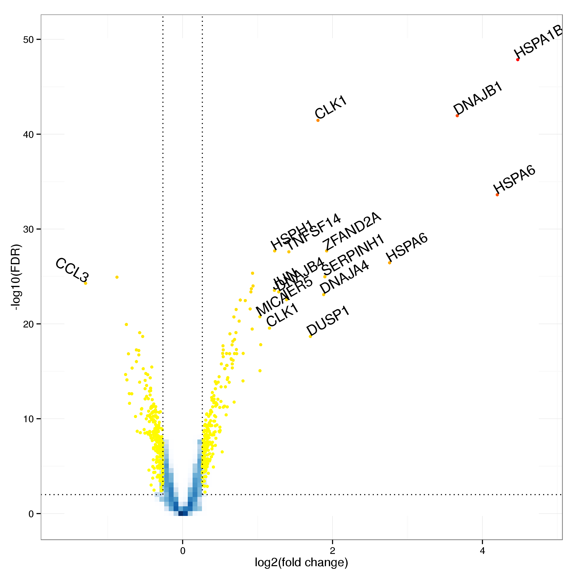
Figure 9: Volcano plot of differential expression results. Probes with an adjusted p-value below 0.01 and a log fold cange of at least 0.5 are shown as yellow and red dots. Probes showing particularly strong evidence of changes in gene expression through a combination of p-value and fold change are labelled with the corresponding gene symbol.

sortedTable <- dplyr::arrange(dplyr::filter(limmaTable, adj.P.Val < fdrCut, 
    abs(logFC) > fcCut), desc(logFC))
sideCols <- c(Basal = "purple", Stim = "orange")
treat <- str_extract(colnames(sig.data.norm), "(Basal|Stim)$")
heatmap.2(sig.data.norm[sortedTable$ArrayAddress, ], trace = "none", Rowv = FALSE, 
    Colv = TRUE, scale = "row", dendrogram = "column", col = rev(brewer.pal(11, 
        "RdBu")), ColSideColors = sideCols[treat], key = FALSE, labRow = "", 
    labCol = "", xlab = "Samples", ylab = "Genes")

**Figure 10:** Heatmap comparing gene expression for differentially expressed genes between basal and stimulated samples. Samples were clustered by gene  with stimulated (orange) and basal (purple) samples forming two distinct groups. Expression estimates for each gene were scaled and centred across samples. Blue cells correspond to lower and red cells to higher than average expression.

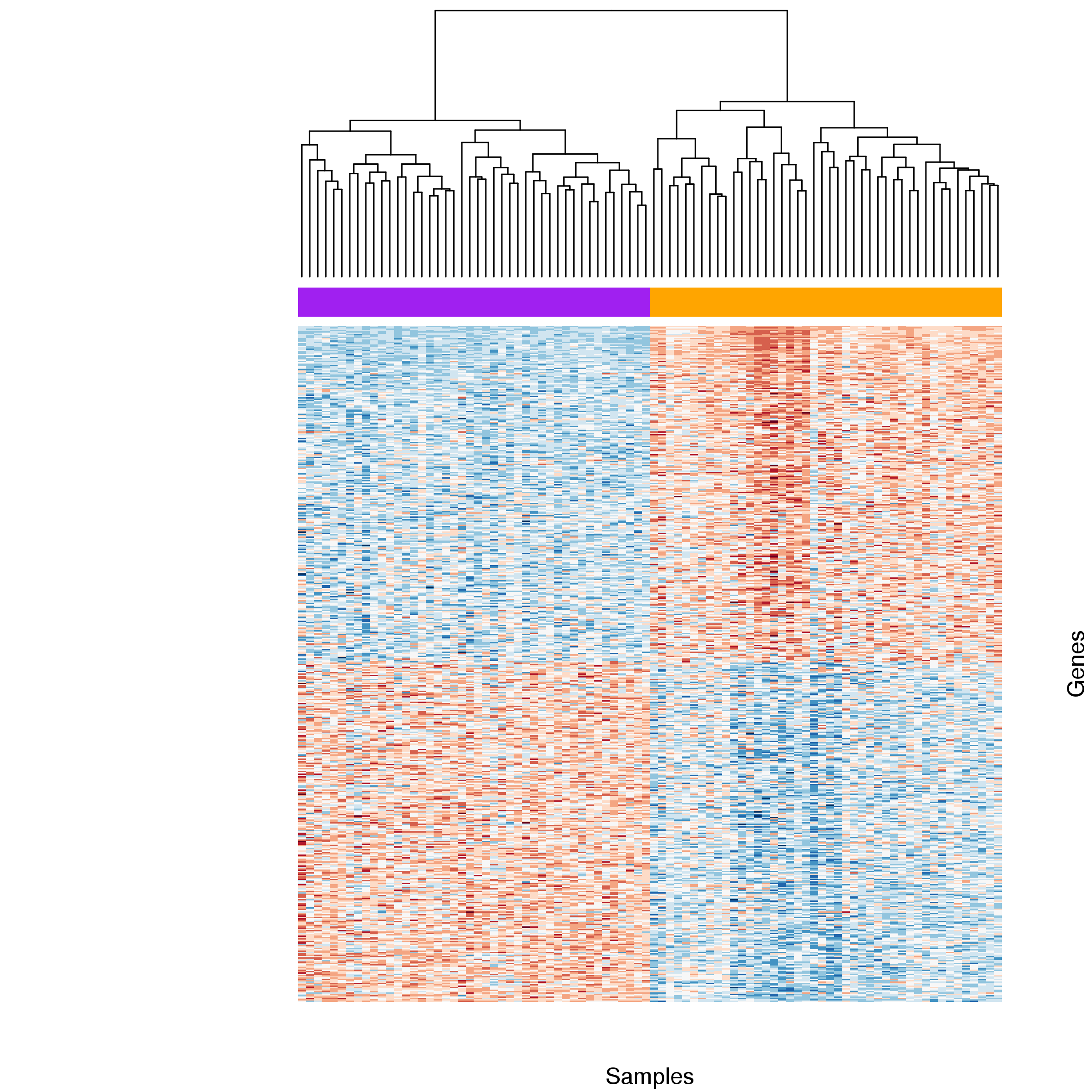
Figure 10: Heatmap comparing gene expression for differentially expressed genes between basal and stimulated samples. Samples were clustered by gene with stimulated (orange) and basal (purple) samples forming two distinct groups. Expression estimates for each gene were scaled and centred across samples. Blue cells correspond to lower and red cells to higher than average expression.

GO enrichment analysis

The GO analysis highlights several categories that are significantly enriched among the up and down regulated genes (7 and 0 categories with an FDR < 0.05 respectively). Considering the top categories (Table 4 and Table 5) it appears that genes up regulated in response to heat shock are predominantly related to stress response (including response to heat [GO:0009408]) and protein folding (including response to unfolded protein [GO:0006986] and protein refolding [GO:0042026]) whereas the leading GO categories for down regulated genes broadly relate to cell proliferation and normal lymphocyte function and include positive regulation of cell cycle [GO:0045787], spindle assembly [GO:0051225] and chemokine production [GO:0032602] but are not sufficiently enriched to be considered significant.

set.caption(tabRef("topGOUp", "Top 20 GO categories enriched for up regulated genes."))
pander(head(dplyr::select(goTabUp, -up, -down), 20))
Table 5: Top 20 GO categories enriched for up regulated genes.
GO.IDTermAnnotatedSignificantExpectedRank in downup FDRdown FDR
GO:0009408response to heat70131.524830.0002261
GO:0006986response to unfolded protein97152.0927530.0002731
GO:0006457protein folding133172.8615930.000641
GO:0035966response to topologically incorrect prot…106152.2823620.0009391
GO:0009266response to temperature stimulus96132.0622570.009811
GO:0042026protein refolding1150.2427540.02771
GO:0034605cellular response to heat5091.0727550.0351
GO:0043618regulation of transcription from RNA pol…3570.7519040.1791
GO:1900034regulation of cellular response to heat2660.5627560.2731
GO:0043620regulation of DNA-templated transcriptio…3970.8420080.3671
GO:0090083regulation of inclusion body assembly1040.2127570.4691
GO:0034976response to endoplasmic reticulum stress124122.6726870.7241
GO:0042542response to hydrogen peroxide5881.2527580.8091
GO:0080135regulation of cellular response to stres…303206.51146711
GO:0043066negative regulation of apoptotic process425259.14126711
GO:0070841inclusion body assembly1340.28275911
GO:0043069negative regulation of programmed cell d…428259.2129911
GO:0060548negative regulation of cell death459269.8756311
GO:0036003positive regulation of transcription fro…1440.3276011
GO:1902175regulation of oxidative stress-induced i…1540.32276111
set.caption(tabRef("topGODown", "Top 20 GO categories enriched for down regulated genes"))
pander(head(dplyr::select(goTabDown, -up, -down), 20))
Table 6: Top 20 GO categories enriched for down regulated genes
GO.IDTermAnnotatedSignificantExpectedRank in upup FDRdown FDR
GO:0051225spindle assembly3760.82272311
GO:0043207response to external biotic stimulus342207.56191711
GO:0051707response to other organism342207.56191811
GO:0007049cell cycle10374522.9204611
GO:0045931positive regulation of mitotic cell cycl…6471.41272411
GO:0007143female meiotic division1030.22272511
GO:0009607response to biotic stimulus355207.85171111
GO:0032496response to lipopolysaccharide128102.83158211
GO:1903047mitotic cell cycle process5522712.2225111
GO:0008219cell death10224322.64411
GO:0002237response to molecule of bacterial origin134102.96166211
GO:0016265death10254322.73611
GO:0001819positive regulation of cytokine producti…180123.985711
GO:0006353DNA-templated transcription, termination5761.26155911
GO:0000278mitotic cell cycle6272913.9223611
GO:1901654response to ketone6061.3368811
GO:0022402cell cycle process7833417.3208711
GO:0000226microtubule cytoskeleton organization213134.71259311
GO:0000070mitotic sister chromatid segregation8071.77200411
GO:0051726regulation of cell cycle5572612.3186511
tblUp <- GenTable(tg$up, cluster1 = resultUp, topNodes = length(score(resultUp)))
tblUp$cluster1 <- as.numeric(tblUp$cluster1)
tblDown <- GenTable(tg$down, cluster2 = resultDown, topNodes = length(score(resultDown)))
tblDown$cluster2 <- as.numeric(tblDown$cluster2)
tbl <- bind_rows(gather(tblUp, "direction", "p.value", cluster1), gather(tblDown, 
    "direction", "p.value", cluster2))
## Warning in rbind_all(list(x, ...)): Unequal factor levels: coercing to
## character
ggplot(tbl, aes(x = Expected, y = Significant)) + geom_point(data = dplyr::filter(tbl, 
    p.value >= 1e-04), colour = "grey") + geom_point(data = dplyr::filter(tbl, 
    p.value < 1e-04), aes(fill = -log10(p.value), shape = direction), size = 2.5) + 
    geom_abline(intercept = 0, slope = 1) + scale_shape_manual(values = c(up = 24, 
    down = 25)) + theme_bw()
## Warning: Removed 10 rows containing missing values (geom_point).

**Figure 11:** GO category enrichment for differentially expressed genes.

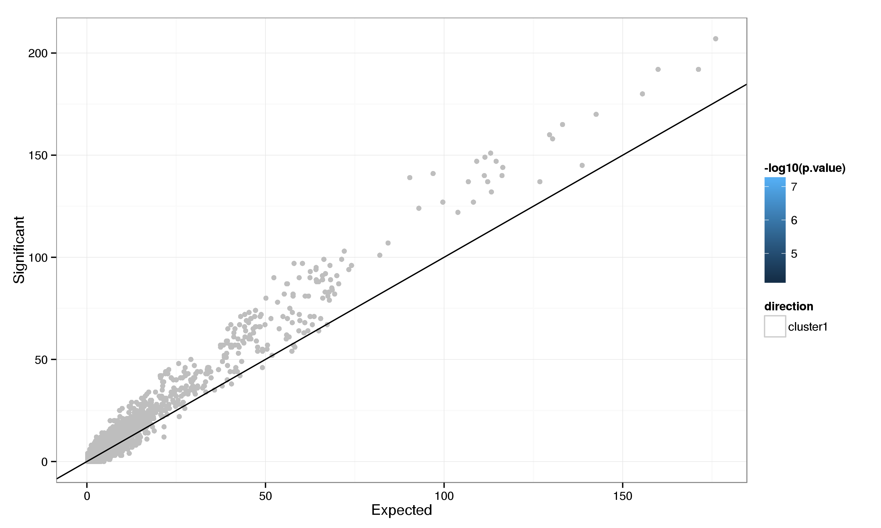
Figure 11: GO category enrichment for differentially expressed genes.

Gene annotations

Of the 226 significantly up regulated genes 24 have been directly linked to the heat shock response and 98 are associated with GO terms that clearly relate to heat shock response (Fisher’s exact test P-value: 2.36e-10) and a further 21 are otherwise linked to the heat shock response in the literature. This leaves 83 genes with no obvious association to heat shock. Using a more inclusive definition of heat shock related processes, also including GO terms related to cell death and proliferation, accounts for an additional 30 genes, leaving 53 genes without any known heatshock association.

condition <- str_replace(hsfPval$cond, "comb-C_", "basal ")
condition <- str_replace(condition, "comb-HS_", "heat shock ")
tab <- data.frame(Condition = condition, up = paste0(hsfPval$sigGenes_up, " (P=", 
    format(hsfPval$up, digits = 2), ", OR=", format(hsfPval$up.or, digits = 2), 
    ")"), down = paste0(hsfPval$sigGenes_down, " (P=", format(hsfPval$down, 
    digits = 2), ", OR=", format(hsfPval$down.or, digits = 2), ")"))
tab$up <- str_replace(tab$up, fixed("e+00"), "")
tab$down <- str_replace(tab$down, fixed("e+00"), "")
tab$up <- sub("\\(([[:digit:]]\\.[[:digit:]])e(-[[:digit:]]+)\\)", "\\$(\\1 \\\\times 10^{\\2})\\$", 
    tab$up)

set.caption(tabRef("peakEnrich", "Number (and corresponding p-values) of ChIP-seq peaks for HSF1 and HSF2 associated with significantly up and down regulated genes."))
highlightStrong <- NULL
if (any(hsfPval$up < 0.001)) highlightStrong <- cbind(which(hsfPval$up < 0.001), 
    2)
if (any(hsfPval$down < 0.001)) highlightStrong <- rbind(highlightStrong, cbind(which(hsfPval$down < 
    0.001), 3))

highlight <- NULL
if (any(hsfPval$up < 0.01 & hsfPval$up > 0.001)) highlight <- cbind(which(hsfPval$up < 
    0.01 & hsfPval$up > 0.001), 2)
if (any(hsfPval$down < 0.01 & hsfPval$down > 0.001)) highlight <- rbind(highlight, 
    cbind(which(hsfPval$down < 0.01 & hsfPval$down > 0.001), 3))

pander(tab, emphasize.cells = highlight, emphasize.strong.cells = highlightStrong)
Table 7: Number (and corresponding p-values) of ChIP-seq peaks for HSF1 and HSF2 associated with significantly up and down regulated genes.
Conditionupdown
basal HSF11 (P=4.3e-01, OR= 1.8)0 (P=1.00, OR=0.00)
basal HSF27 (P=9.6e-03, OR= 3.2)2 (P=0.71, OR=0.81)
heat shock HSF151 (P=4.7e-10, OR= 3.0)6 (P=1.00, OR=0.31)
heat shock HSF255 (P=9.4e-09, OR= 2.6)10 (P=1.00, OR=0.43)
basal HSF1+HSF21 (P=8.6e-02, OR=14.7)0 (P=1.00, OR=0.00)
heat shock HSF1+HSF246 (P=9.1e-15, OR= 4.5)4 (P=1.00, OR=0.34)

There are 7 up-regulated genes without any established role, 8 genes with limited evidence and 29 with substantial evidence for their involvement in the heat shock response that show heat shock factor binding in their promoter region. Further evidence for the binding of HSF1 and HSF2 in these regions is provided by scanning for the presence of the HSF1 binding motif. While this provides less direct evidence than the presence of a ChIP-seq peak and even a good match for the motif is no guarantee for the presence of an active binding site, it enables the detection of potential binding sites that may be inactive in the cell type or state studied through ChIP-seq experiments. Although overall the evidence for the presence of the HSF1 motif is relatively weak, there is a clear increase in the average score for genes that show evidence of HSF binding compared to those that don’t (Figure 12).

ggplot(dplyr::filter(r_gene, expr == "up"), aes(x = factor(HSFpeak, levels = c("0", 
    "1"), labels = c("absent", "present")), y = -log10(pwm.p.value), fill = factor(novel, 
    levels = c("0", "1", "2", "3"), labels = c("established", "strong", "limited", 
        "novel")))) + geom_boxplot() + theme_bw() + xlab("HSF peak") + ylab(expression(-log[10]("p-value"))) + 
    scale_fill_discrete(name = "heat shock association")

**Figure 12:** Distribution of p-values for HSF1 motif score.

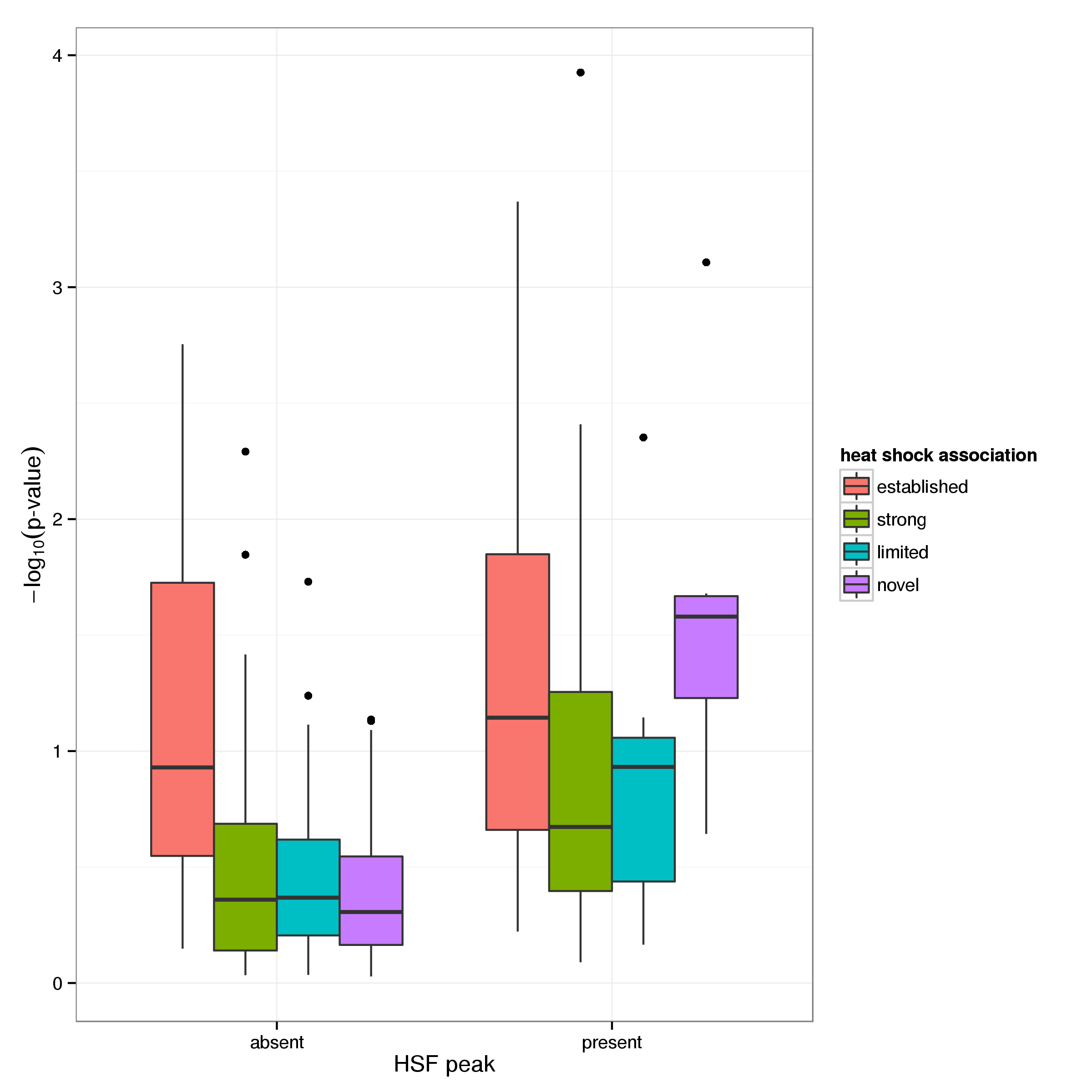
Figure 12: Distribution of p-values for HSF1 motif score.

hsfTab <- data.frame(expression = r_gene$expr, ChIPseq = ifelse(r_gene$HSFpeak == 
    1, "yes", "no"), motif = ifelse(r_gene$pwm.p.value < 0.05, "present", "absent"))
tab <- tidyr::spread(as.data.frame(table(hsfTab)), motif, Freq)
tab[["frequency"]] <- paste0(sprintf("%0.2f", tab$present/(tab$present + tab$absent) * 
    100), "%")

upTest <- fisher.test(tab[tab$expression == "up", c("absent", "present")], alternative = "greater")
downTest <- fisher.test(tab[tab$expression == "down", c("absent", "present")], 
    alternative = "greater")

set.caption(tabRef("HSFtable", "Summary of HSF1 motif occurance in promoters of differentially expressed genes. with and without HSF ChIP-seq peaks."))
pander(tab)
Table 8: Summary of HSF1 motif occurance in promoters of differentially expressed genes. with and without HSF ChIP-seq peaks.
expressionChIPseqabsentpresentfrequency
upno15595.49%
upyes431728.33%
downno206177.62%
downyes9325.00%
othersno74667769.42%
othersyes40710019.72%

Considering the frequency with wich HSF1 motifs occur (using a p-value threshold of 0.05) in the promoter regions of genes with and without ChIP-seq binding evidence (Table 8) it is apparent that the motif is enriched amongst up-regulated genes with corresponding protein binding evidence (Fisher’s exact test p-value: 1.2e-05). This enrichment is less pronounced for down regulated genes (0.071).

Further examining up-regulated genes for evidence of HSF binding reveals that 8 genes not previously characterised as heat shock response genes have ChIP-seq peaks and of these 1 also carry the HSF1 binding motif in their promoter (Table 9 and Table 10).

hsfTab$type <- ifelse(r_gene$novel == 2, "novel", ifelse(r_gene$novel == 1, 
    "limited", "established"))
hsfTab <- dplyr::filter(hsfTab, expression == "up") %>% dplyr::select(-expression)
tab <- tidyr::spread(as.data.frame(table(hsfTab)), type, Freq)

set.caption(tabRef("HSFnovel", "Summary of HSF binding evidence for the promoters of novel and established heat shock response genes."))
pander(tab, emphasize.strong.cells = matrix(c(3, 4, 5, 5), ncol = 2))
Table 9: Summary of HSF binding evidence for the promoters of novel and established heat shock response genes.
ChIPseqmotifestablishedlimitednovel
noabsent498521
nopresent351
yesabsent13237
yespresent1061
set.caption(tabRef("novelTable", "Genes with newly established links to heat shock response"))
tab <- dplyr::filter(r_gene, novel == 2, HSFpeak == 1) %>% dplyr::select(`Gene Symbol` = SymbolReannotated, 
    `Fold Change` = logFC, `expression FDR` = adj.P.Val, `Motif p-value` = pwm.p.value) %>% 
    dplyr::arrange(desc(`Fold Change`), `Motif p-value`)
tab[["Fold Change"]] <- 2^tab[["Fold Change"]]
pander(tab)
Table 10: Genes with newly established links to heat shock response
Gene SymbolFold Changeexpression FDRMotif p-value
NAA161.574.77e-170.683
USPL11.541.44e-140.00444
FAM46A1.53.92e-110.32
GPBP11.361.15e-080.108
TYW31.331.82e-100.0937
EARS21.311.11e-120.0716
MTCH11.225.38e-100.127
TRMT1121.224.38e-070.543

Global heat shock response

Considering the outcome of the partial least squares regression it is apparent that there is a considerable change in overall gene expression in response to heat shock. Together the first two PLS components account for 96.1% in the variation observed due to heat shock and provide clear separation of the two treatment groups (Figure 13).

plsComp <- cbind(plsComp, sex = factor(globalPheno[plsComp$sample, "sex"]))
fig1 <- plsPlot(plsComp, group = c("treatment", "cluster"))
fig2 <- ggdendrogram(plsClust) + geom_hline(yint = cutHeight, col = "red")
multiplot(fig1, fig2, cols = 2)

**Figure 13:** Samples separate clearly by treatment, showing a consistent global effect on gene expression from heat shock. Stimulated samples show evidence of three distinct groups.

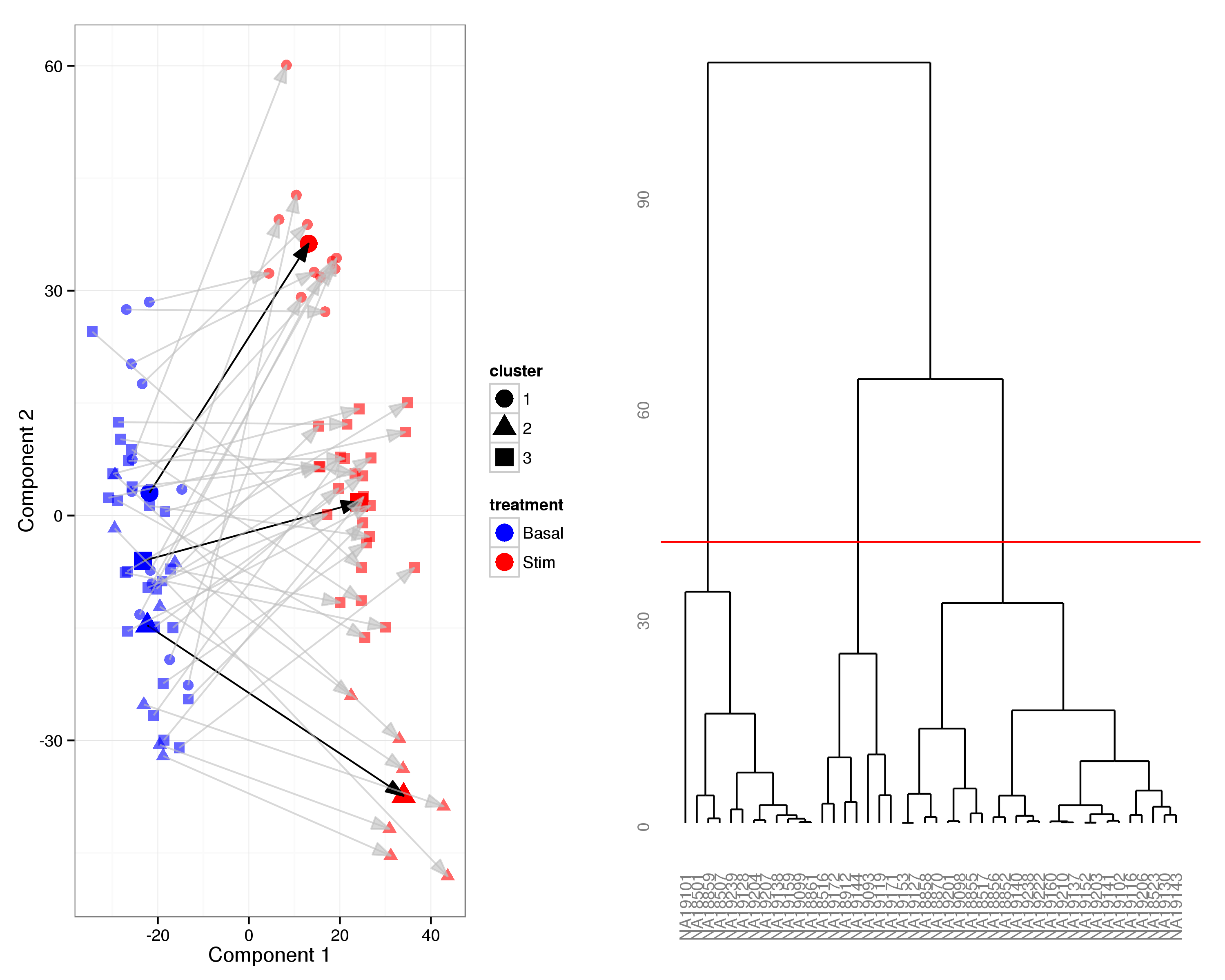
Figure 13: Samples separate clearly by treatment, showing a consistent global effect on gene expression from heat shock. Stimulated samples show evidence of three distinct groups.

Of the 19732 SNPs tested for association with the global response phenotype 2 are considered significant (FDR < 0.05) (Table 11). These SNPs form 2 group of highly correlated genotypes, likely due to local LD structure.

sel <- which(assoc$adj.p.val < 0.1)
coef <- assoc$Results[sel, , 1]
coef[, "JointModel"] <- assoc$adj.p.val[sel]
colnames(coef)[ncol(coef)] <- "Joint model FDR"
set.caption(tabRef("treatPLS", "Standardised coefficients and adjusted p-values for the top SNPs."))
pander(coef)
Table 11: Standardised coefficients and adjusted p-values for the top SNPs.
 basal.xbasal.ydirectiondistanceJoint model FDR
rs10509407-4.78-4.52-0.332-4.710.021
rs12259569-4.78-4.85-0.576-4.510.025
rs122075481.260.4521.870.9250.064
rs7012294-0.543-2.26-2.51-3.010.066

fig1 <- ggplot(data.frame(p.value = pPerm[, bins[dimnames(assoc$Result)[[1]][1]]]), 
    aes(x = -log10(p.value))) + geom_histogram(fill = "lightgrey", binwidth = 0.1) + 
    geom_vline(xintercept = -log10(assoc$Results[1, "JointModel", 2]), colour = "red") + 
    theme_bw() + xlab(expression(-log[10]("p-value")))

fig2 <- ggplot(data.frame(p.value = apply(pPerm, 1, min)), aes(x = -log10(p.value))) + 
    geom_histogram(fill = "lightgrey", binwidth = 0.1) + geom_vline(xintercept = -log10(assoc$Results[1, 
    "JointModel", 2]), colour = "red") + theme_bw() + xlab(expression(-log[10]("p-value")))

fig3 <- ggplot(data.frame(p.value = pPerm[, bins[dimnames(assoc$Result)[[1]][3]]]), 
    aes(x = -log10(p.value))) + geom_histogram(fill = "lightgrey", binwidth = 0.1) + 
    geom_vline(xintercept = -log10(assoc$Results[3, "JointModel", 2]), colour = "red") + 
    theme_bw() + xlab(expression(-log[10]("p-value")))

fig4 <- ggplot(data.frame(p.value = apply(pPerm, 1, min)), aes(x = -log10(p.value))) + 
    geom_histogram(fill = "lightgrey", binwidth = 0.1) + geom_vline(xintercept = -log10(assoc$Results[3, 
    "JointModel", 2]), colour = "red") + theme_bw() + xlab(expression(-log[10]("p-value")))


multiplot(fig1, fig2, fig3, fig4, layout = matrix(1:4, ncol = 2, byrow = TRUE))

**Figure 14:** P-values observed after permutation of global response phenotype for SNPs rs10509407 (top) and rs12207548 (bottom). The distribution of p-values for each snp after permutation is shown on the left and the minimum p-value observed in each iteration across all SNPs on the right.

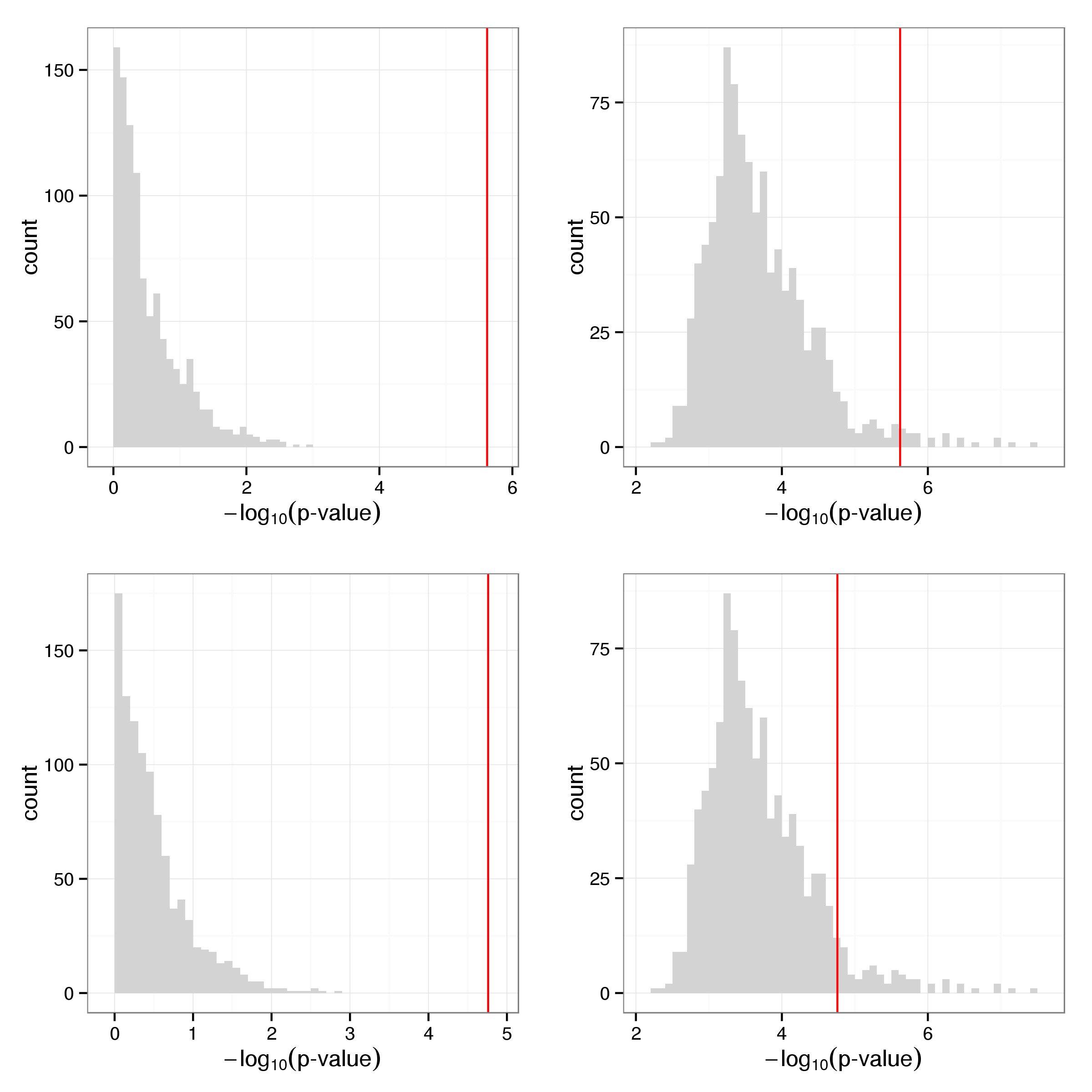
Figure 14: P-values observed after permutation of global response phenotype for SNPs rs10509407 (top) and rs12207548 (bottom). The distribution of p-values for each snp after permutation is shown on the left and the minimum p-value observed in each iteration across all SNPs on the right.

Figure 15 shows two examples of genotypes associating with the global heat shock response. Note that the second one (rs12207548) is located within a CTCF binding site immediately downstream of CDKN1A, an important regulator of cell cycle progression. This SNP is also found to be associated with the expession level of HSF1 in resting lymphocytes (Table 12) It may be interesting to note that allele frequencies vary markedly across populations. While the frequency of the ancestral T allele is 79% in the Yoruba 1000 genomes samples it is only observed with a frequency of 24% in European samples.

genotypes <- data.frame(sample = colnames(geno$bed), stringsAsFactors = FALSE)
genotypes <- cbind(genotypes, t(geno$bed[dimnames(assoc$Results)[[1]][sel], 
    ]))
plsComp <- dplyr::left_join(plsComp, genotypes, by = "sample")

fig1 <- plsPlot(plsComp, dimnames(assoc$Results)[[1]][1]) + guides(colour = "none")
fig2 <- plsPlot(plsComp, dimnames(assoc$Results)[[1]][3]) + guides(colour = "none")
multiplot(fig1, fig2, cols = 2)

**Figure 15:** Global response to heat shock by genotype for rs10509407 (left) and rs12207548 (right). Each individual is represented by two points corresponding to basal and stimulated state with arrows connecting paired samples. Genotypes are indicated by colour with blue corresponding to homozyguous carriers of the major allele and red indicating the presence of at least one minor allele.

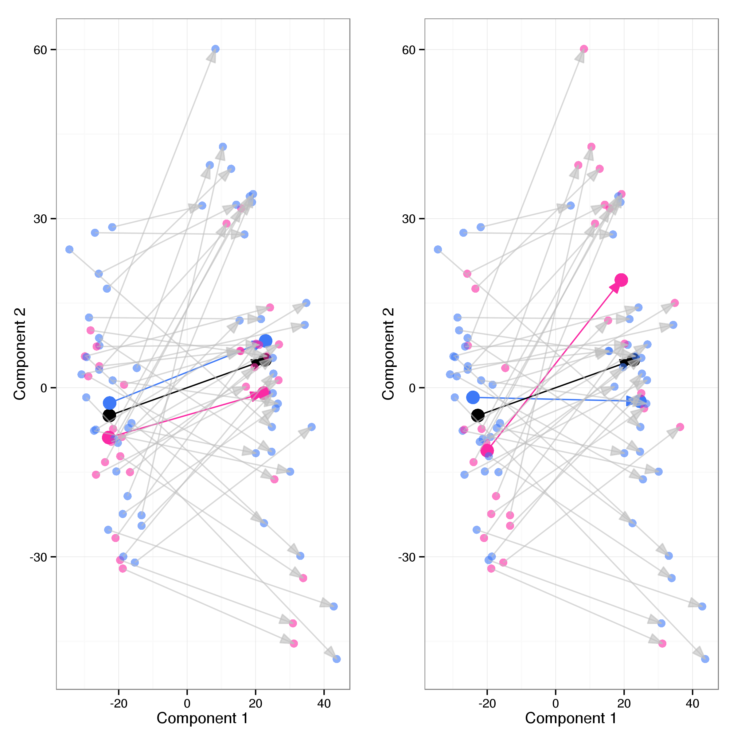
Figure 15: Global response to heat shock by genotype for rs10509407 (left) and rs12207548 (right). Each individual is represented by two points corresponding to basal and stimulated state with arrows connecting paired samples. Genotypes are indicated by colour with blue corresponding to homozyguous carriers of the major allele and red indicating the presence of at least one minor allele.

tab <- meGlobal$all$eqtls
n <- max(sum(tab$FDR < 0.05), 5)
cut <- tab$FDR[n]
n <- min(max(which(tab$FDR <= cut)), 20)

tab <- dplyr::left_join(tab, dplyr::select(limmaTable, NuID, SymbolReannotated), 
    by = c(gene = "NuID"))
## Warning in left_join_impl(x, y, by$x, by$y): joining character vector and
## factor, coercing into character vector
tab <- dplyr::rename(tab, Gene = SymbolReannotated)
tab <- dplyr::select(tab, SNP = snps, Gene, NuID = gene, Statistic = statistic, 
    `p-value` = pvalue, FDR, beta)
set.caption(tabRef("globalSNPGenes_fc", "Associations between global response SNPs and gene level heat shock response."))
pander(dplyr::select(head(tab, n), -NuID))
Table 13: Associations between global response SNPs and gene level heat shock response.
SNPGeneStatisticp-valueFDRbeta
rs12207548TNFRSF8-5.413.21e-060.000751-0.477
rs12207548HSF1-5.353.84e-060.000751-0.643
rs12207548EPHB1-5.255.34e-060.000751-0.532
rs12207548SHC1-4.722.92e-050.00308-0.456
rs12207548ZC3HAV1-4.64.25e-050.00358-0.399
rs12207548ACBD3-4.170.0001570.0102-0.279
rs12207548UBQLN1-4.150.0001690.0102-0.238
rs10509407UBQLN14.070.0002160.01140.232
n <- sum(tab$FDR < 0.05)
if (n < 2) n <- 2
fig <- vector(mode = "list", n)

for (i in 1:n) {
    snp <- as.character(tab$SNP[i])
    gene <- as.character(tab$Gene[i])
    probe <- as.character(tab$NuID[i])
    
    fit <- lm(selectedFC[probe, ] ~ geno$bed[snp, ] + t(covar[[1]]))
    offset <- colSums(fit$coefficients[-(1:2)] * covar[[1]])
    
    plotData <- data.frame(genotype = geno$bed[snp, ], fold_change = selectedFC[probe, 
        ] - offset)
    fig[[i]] <- ggplot(plotData, aes(x = factor(genotype), y = fold_change)) + 
        geom_point(position = position_jitter(width = 0.1), size = 2.5) + geom_boxplot(alpha = 0.4, 
        outlier.colour = "white", fill = "grey") + theme_bw() + xlab(snp) + 
        ylab(paste(gene, "(log fold change)"))
}
cols <- 1
if (n > 1) cols <- 2
if (n > 4) cols <- 3
multiplot(plotlist = fig, cols = cols)

**Figure 16:** Heat shock response by genotype.

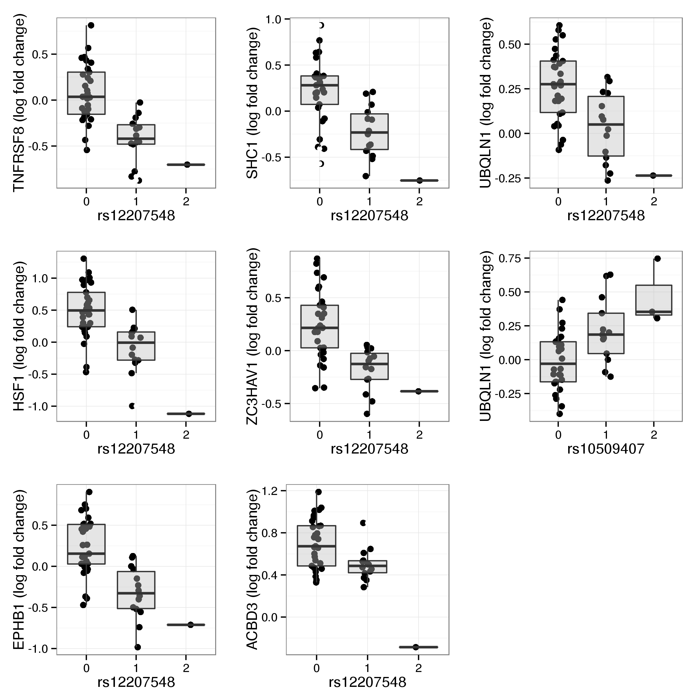
Figure 16: Heat shock response by genotype.

tab <- meGlobalStim$all$eqtls
cut <- tab$FDR[5]
n <- min(max(which(tab$FDR <= cut)), 20)
tab <- head(tab, n)
tab <- dplyr::left_join(tab, dplyr::select(limmaTable, NuID, SymbolReannotated), 
    by = c(gene = "NuID"))
## Warning in left_join_impl(x, y, by$x, by$y): joining character vector and
## factor, coercing into character vector
tab <- dplyr::select(tab, -gene) %>% dplyr::rename(Gene = SymbolReannotated)
tab <- dplyr::select(tab, SNP = snps, Gene, Statistic = statistic, `p-value` = pvalue, 
    FDR, beta)
set.caption(tabRef("globalSNPGenes_stim", "Associations between global response SNPs and gene expression following heat shock."))
pander(tab)
Table 14: Associations between global response SNPs and gene expression following heat shock.
SNPGeneStatisticp-valueFDRbeta
rs12207548HSPA1B3.520.001110.4670.304
rs12207548PPP5C2.80.007870.9260.204
rs12207548RSRC2-2.650.01160.926-0.166
rs10509407EGR12.480.01760.9260.178
rs10509407HSPA42.460.01830.9260.126
rs12207548HSPA42.390.02180.9260.153
rs10509407FAS-2.30.02710.926-0.147
rs10509407E2F32.190.03420.9260.114
rs10509407UBQLN12.190.03450.9260.0915
rs12207548HSF1-2.170.03590.926-0.171
rs12207548PRR7-2.170.03620.926-0.177
rs10509407MAPK142.120.040.9260.106
rs12207548PRKCE-2.080.04450.926-0.158
rs12207548ZFAND2A2.060.0460.9260.199
rs12207548NEDD92.050.04720.9260.141
rs12207548SPR2.030.04920.9260.276
rs12207548FAS2.020.05040.9260.163
rs10509407TNFSF14-1.950.05830.926-0.171
rs12207548SHC1-1.910.06290.926-0.164
rs12207548GPR89A-1.910.0630.926-0.0985
tab <- meGlobalBasal$all$eqtls
cut <- tab$FDR[5]
n <- min(max(which(tab$FDR <= cut)), 20)
tab <- head(tab, n)
tab <- dplyr::left_join(tab, dplyr::select(limmaTable, NuID, SymbolReannotated), 
    by = c(gene = "NuID"))
## Warning in left_join_impl(x, y, by$x, by$y): joining character vector and
## factor, coercing into character vector
tab <- dplyr::select(tab, -gene) %>% dplyr::rename(Gene = SymbolReannotated)
tab <- dplyr::select(tab, SNP = snps, Gene, Statistic = statistic, `p-value` = pvalue, 
    FDR, beta)
set.caption(tabRef("globalSNPGenes_basal", "Associations between global response SNPs and gene expression in basal state."))
pander(tab)
Table 12: Associations between global response SNPs and gene expression in basal state.
SNPGeneStatisticp-valueFDRbeta
rs12207548HSF14.230.0001380.05820.341
rs12207548FOSL13.580.000940.1980.159
rs10509407NR3C1-3.370.00170.239-0.154
rs10509407UBQLN1-3.140.003230.311-0.14
rs12207548ZC3HAV13.010.004610.3110.203
rs12207548SHC12.960.005220.3110.182
rs12207548TCP12.920.005810.3110.186
rs12207548BANP-2.860.006770.311-0.154
rs12207548TRAF22.850.006860.3110.162
rs10509407MTCH1-2.750.008970.311-0.105
rs10509407USPL12.720.00960.3110.119
rs12207548GNB1-2.680.01060.311-0.132
rs12207548JUN-2.680.01070.311-0.266
rs10509407PADI42.680.01080.3110.121
rs10509407UBQLN12.670.01110.3110.101

Noting that the minor allele frequency of rs12207548 varies considerably between populations we thought to investigate wether there is evidence of selection at this locus. To this end we calculated FST between the Yoruban and Central European populations for this SNP and compare it to all SNPs with similar MAF in the Yoruban samples.

yri <- getSS("hmyriB36", paste0("", 1:22))
yri <- yri[, phenoData(yri)$isFounder == 1]
yri <- MAFfilter(yri, 0.17, 0.21)
geno.yri <- smList(yri)

ceu <- getSS("ceuhm3", paste0("chr", 1:22))
ceu <- ceu[, phenoData(ceu)$isFounder == 1]
geno.ceu <- smList(ceu)
geno.ceu <- mapply(function(x, y) {
    snps <- colnames(y)
    snps <- snps[snps %in% colnames(x)]
    x[, snps]
}, geno.ceu, geno.yri, SIMPLIFY = FALSE)
geno.yri <- mapply(function(x, y) {
    snps <- colnames(y)
    snps <- snps[snps %in% colnames(x)]
    x[, snps]
}, geno.yri, geno.ceu, SIMPLIFY = FALSE)
fst <- mapply(function(x, y) Fst(rbind(x, y), rep(c("ceu", "yri"), c(nrow(x), 
    nrow(y))))$Fst, geno.ceu, geno.yri, SIMPLIFY = FALSE)
fst <- unlist(fst)
names(fst) <- unlist(lapply(geno.yri, colnames))

This estimates the FST for rs12207548 to be 0.31. Of the 1175115 SNPs tested 10.55% have a more extreme value.

Investigating the differences in gene expression between cluster 1 and 2 of the second PLS component we identified a total of 1096 probes as differentially expressed at an FDR threshold of 0.01 (see Table 15 for the top 20 results). Of these 681 are up and 415 down regulated in cluster 2 compared to expression levels in cluster 1. Almost all of these (1094) have a fold change of at least 1.2. Figure 17 shows a smoothed volcano plot highlighting probes of particular interest.

set.caption(tabRef("clusterTopTable", "Top 20 differentially expressed probes."))
rownames(clust1_2Table) <- NULL
pander(head(dplyr::select(clust1_2Table, -ArrayAddress, -EntrezReannotated, 
    -GenomicLocation), 20))
Table 15: Top 20 differentially expressed probes.
NuIDSymbolReannotatedlogFCAveExprtP.Valueadj.P.ValB
Z5UZO6CcrqHT1w95b4MED220.8559.2810.91.69e-142.1e-1022.6
ltLUV5VtR.VN12swNMTOMM400.9311.910.21.42e-138.84e-1020.5
WV5XUSD6vUKnvUhB5QGNAI2-1.0910.5-9.638.95e-133.7e-0918.8
rlHpSl1Skrv870kMCsZC3H30.7268.778.997.42e-121.62e-0816.8
HS7hLlJQ7kiujit_4AAIMP20.77911.28.987.69e-121.62e-0816.8
B_gkHi0cdQCrXnUl6cC1orf1120.9038.818.987.81e-121.62e-0816.7
x7leKemno5ulDACSFwINF21.279.568.741.75e-113.11e-0816
or3hBLFTVUSxV9J0v0BCL7B0.9778.138.632.59e-114.02e-0815.6
WebhLrV3VaH5H71_.UPUF600.96711.28.425.25e-117.24e-0814.9
rOezhdXiRW4eVTn9V8RANGAP11.0410.98.288.53e-119.84e-0814.5
Zhq6dHlPtFK_gd_Xe4NOP20.77611.18.278.72e-119.84e-0814.4
9Xop_fqHop_foS9d7sHPS60.9379.668.221.06e-101.1e-0714.2
xKpnfhHuX0.1JUSXq0TYSND10.889.68.181.19e-101.13e-0714.1
lEdet6Oqeefi5IqeawSLC25A191.238.898.061.84e-101.51e-0713.7
01OVCvVK5KEiu6XPsUC17orf530.9828.758.061.84e-101.51e-0713.7
i15CjPunohOJCAJd6gLSP1-1.448.31-8.041.95e-101.51e-0713.7
HzqJNpx567t9VBpGisCD74-1.498.28-7.972.52e-101.84e-0713.4
BesiCOkSjoplUIaEuwE4F11.089.037.913.11e-102.15e-0713.2
NnJ1ITq_NFyKJ3pwpENPRL30.94910.17.814.35e-102.75e-0712.9
upeWHh7uk6JOnvVQuQSNAPC40.7298.97.84.5e-102.75e-0712.9
volcanoPlot(clust1_2Table, fcCut = fcCut, fdrCut = fdrCut)

**Figure 17:** Volcano plot of differential expression results between clusters 1 and 2. Probes with an adjusted p-value below 0.01 and a log fold cange of at least 0.5 are shown as yellow and red dots.

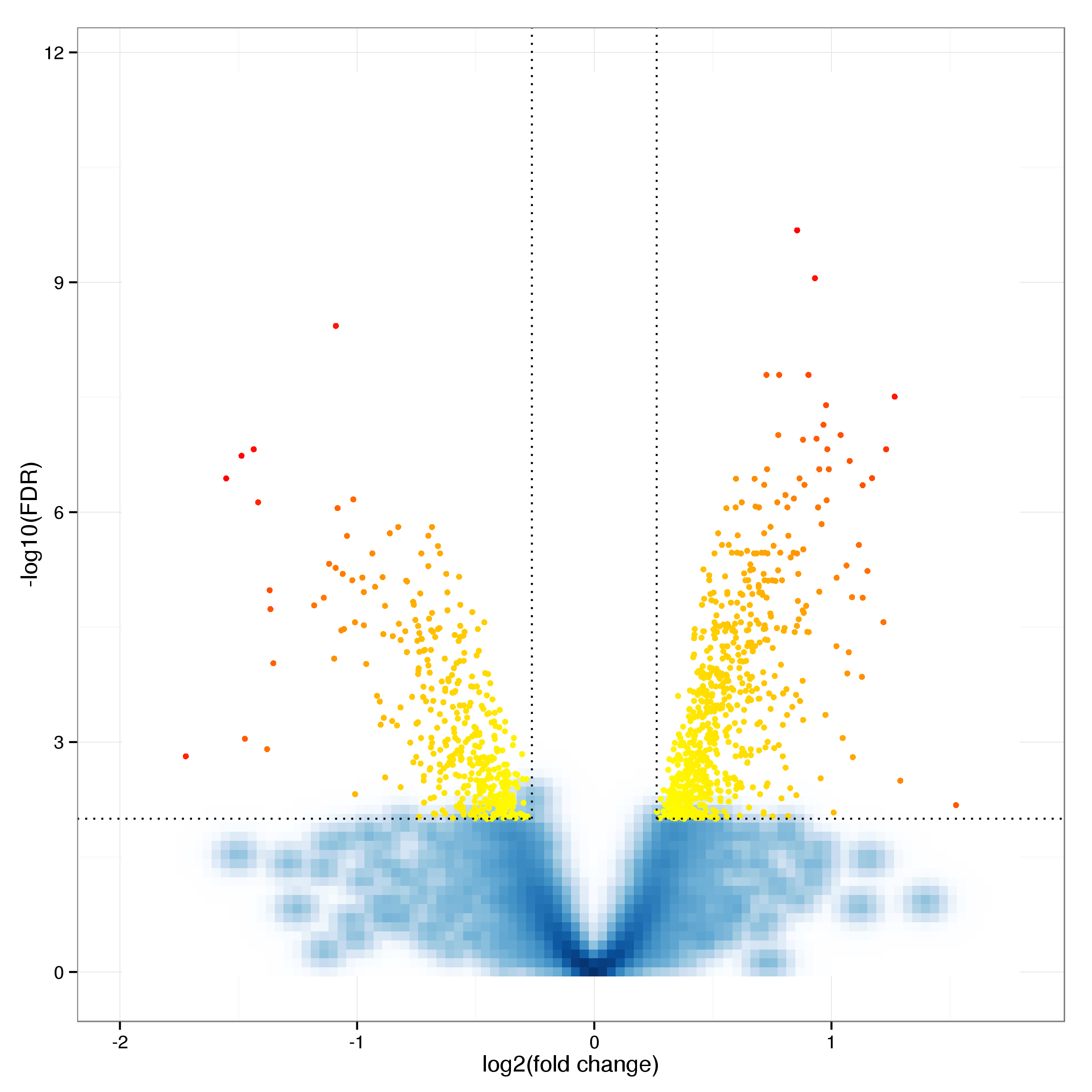
Figure 17: Volcano plot of differential expression results between clusters 1 and 2. Probes with an adjusted p-value below 0.01 and a log fold cange of at least 0.5 are shown as yellow and red dots.

sortedTable <- dplyr::arrange(dplyr::filter(clust1_2Table, adj.P.Val < fdrCut, 
    abs(logFC) > fcCut), desc(logFC))
sideCols <- c(cluster1 = "purple", cluster2 = "orange", cluster3 = "white")
heatmap.2(sig.data.norm[sortedTable$ArrayAddress, plsComp$treatment == "Stim"], 
    trace = "none", Rowv = FALSE, Colv = as.dendrogram(plsClust), dendrogram = "column", 
    scale = "row", col = rev(brewer.pal(11, "RdBu")), ColSideColors = sideCols[plsComp$cluster][plsComp$treatment == 
        "Stim"], key = FALSE, labRow = "", labCol = "", xlab = "Samples", ylab = "Genes")

**Figure 18:** Heatmap comparing gene expression for genes differentially expressed between clusters 1 and 2. Expression estimates for each gene were scaled and centred across samples. Blue cells correspond to lower and red cells to higher than average expression.

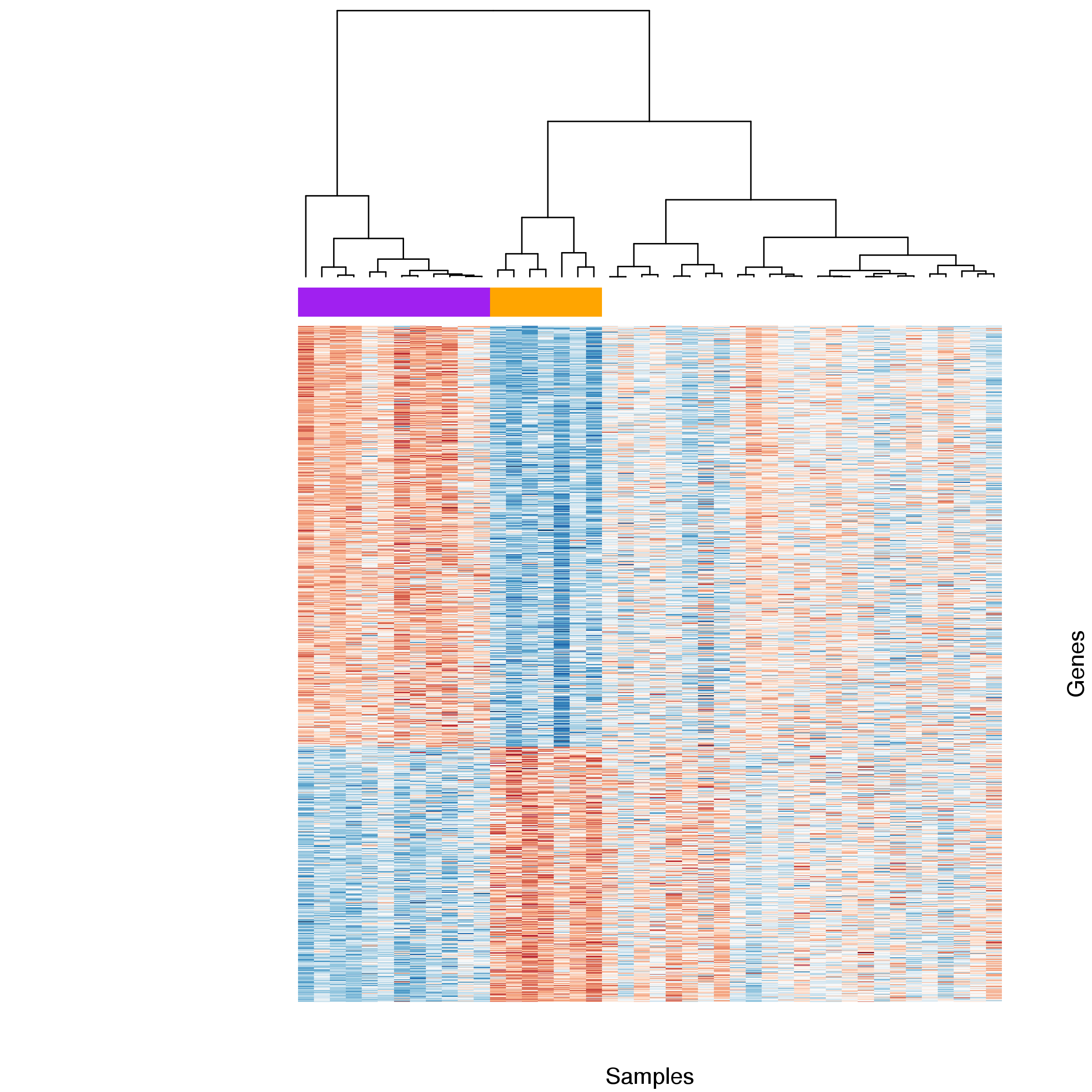
Figure 18: Heatmap comparing gene expression for genes differentially expressed between clusters 1 and 2. Expression estimates for each gene were scaled and centred across samples. Blue cells correspond to lower and red cells to higher than average expression.

goTabPlsUp[["cluster1 FDR"]] <- p.adjust(goTabPlsUp$cluster1)
goTabPlsUp[["cluster2 FDR"]] <- p.adjust(goTabPlsUp$cluster2)
goTabPlsDown[["cluster1 FDR"]] <- p.adjust(goTabPlsDown$cluster1)
goTabPlsDown[["cluster2 FDR"]] <- p.adjust(goTabPlsDown$cluster2)

To further characterise the differnces in gene expression we carried out a GO enrichment analysis for genes differentially expressed between clusters 1 and 2. This reveals strong enrichment for several GO categories (21 and 6 enriched with FDR < 0.05 in cluster 1 and cluster 2 respectively). Genes with increased expression in cluster 1 (Table 16) are enriched for biological processes related to DNA replication whereas those with increased expression in cluster 2 (Table 17) are annotated with processes related to the heat shock response.

set.caption(tabRef("plsTopGOUp", "Top 20 GO categories enriched for genes up regulated in cluster 1"))
pander(dplyr::select(head(goTabPlsUp, 20), -cluster1, -cluster2))
Table 18: Top 20 GO categories enriched for genes up regulated in cluster 1
GO.IDTermAnnotatedSignificantExpectedRank in cluster2cluster1 FDRcluster2 FDR
GO:0034660ncRNA metabolic process2575115.832451.84e-061
GO:0034470ncRNA processing1703810.532521.07e-051
GO:0022613ribonucleoprotein complex biogenesis1984112.232492.69e-051
GO:0042254ribosome biogenesis117297.2132357.26e-051
GO:0006310DNA recombination14633931598.96e-051
GO:0006399tRNA metabolic process96255.9232590.0002471
GO:0006261DNA-dependent DNA replication81214.9929910.003071
GO:0006271DNA strand elongation involved in DNA re…25111.5432600.004691
GO:0022616DNA strand elongation26111.632610.007251
GO:0006281DNA repair276451731830.007671
GO:0006260DNA replication1923511.829750.008521
GO:0006364rRNA processing86215.332050.008951
GO:0000278mitotic cell cycle6278238.732220.009371
GO:0016072rRNA metabolic process88215.4332100.01321
GO:0006312mitotic recombination28111.7332620.01751
GO:0031396regulation of protein ubiquitination134278.2626390.01831
GO:0051340regulation of ligase activity70184.3231390.02131
GO:0006259DNA metabolic process5327132.826810.0231
GO:1903047mitotic cell cycle process552723431570.04251
GO:0051438regulation of ubiquitin-protein transfer…67174.1331320.04681
set.caption(tabRef("plsTopGODown", "Top 20 GO categories enriched for genes up regulated in cluster 2"))
pander(dplyr::select(head(goTabPlsDown, 20), -cluster1, -cluster2))
Table 19: Top 20 GO categories enriched for genes up regulated in cluster 2
GO.IDTermAnnotatedSignificantExpectedRank in cluster1cluster1 FDRcluster2 FDR
GO:0034976response to endoplasmic reticulum stress124204.45259110.00683
GO:0030968endoplasmic reticulum unfolded protein r…74152.66218010.00726
GO:0034620cellular response to unfolded protein74152.66218110.00726
GO:0006986response to unfolded protein97173.48238110.0128
GO:0035967cellular response to topologically incor…81152.91193210.0243
GO:0035966response to topologically incorrect prot…106173.81178010.0427
GO:0032075positive regulation of nuclease activity49111.76183810.064
GO:0032069regulation of nuclease activity53111.9199210.141
GO:0006987activation of signaling protein activity…46101.65169210.213
GO:0080135regulation of cellular response to stres…3033010.9106010.554
GO:1903573negative regulation of response to endop…1860.65337410.554
GO:0009101glycoprotein biosynthetic process206227.4310511
GO:0018196peptidyl-asparagine modification91133.27327911
GO:0018279protein N-linked glycosylation via aspar…91133.27328011
GO:1900101regulation of endoplasmic reticulum unfo…1550.54337511
GO:0031344regulation of cell projection organizati…185206.65255611
GO:1902275regulation of chromatin organization83122.9853811
GO:0006487protein N-linked glycosylation95133.41328811
GO:0045664regulation of neuron differentiation201217.22231611
GO:0045860positive regulation of protein kinase ac…273269.81317011
tblUp <- GenTable(tg_pls$up, cluster1 = resultPlsUp, topNodes = length(score(resultPlsUp)))
tblUp$cluster1 <- as.numeric(tblUp$cluster1)
tblDown <- GenTable(tg_pls$down, cluster2 = resultPlsDown, topNodes = length(score(resultPlsDown)))
tblDown$cluster2 <- as.numeric(tblDown$cluster2)
tbl <- bind_rows(gather(tblUp, "direction", "p.value", cluster1), gather(tblDown, 
    "direction", "p.value", cluster2))
## Warning in rbind_all(list(x, ...)): Unequal factor levels: coercing to
## character
ggplot(tbl, aes(x = Expected, y = Significant)) + geom_point(data = dplyr::filter(tbl, 
    p.value >= 1e-04), colour = "grey") + geom_point(data = dplyr::filter(tbl, 
    p.value < 1e-04), aes(fill = -log10(p.value), shape = direction), size = 2.5) + 
    geom_abline(intercept = 0, slope = 1) + scale_shape_manual(values = c(up = 24, 
    down = 25)) + theme_bw()
## Warning: Removed 51 rows containing missing values (geom_point).

**Figure 19:** GO category enrichment for genes differentially expressed between PLS clusters.

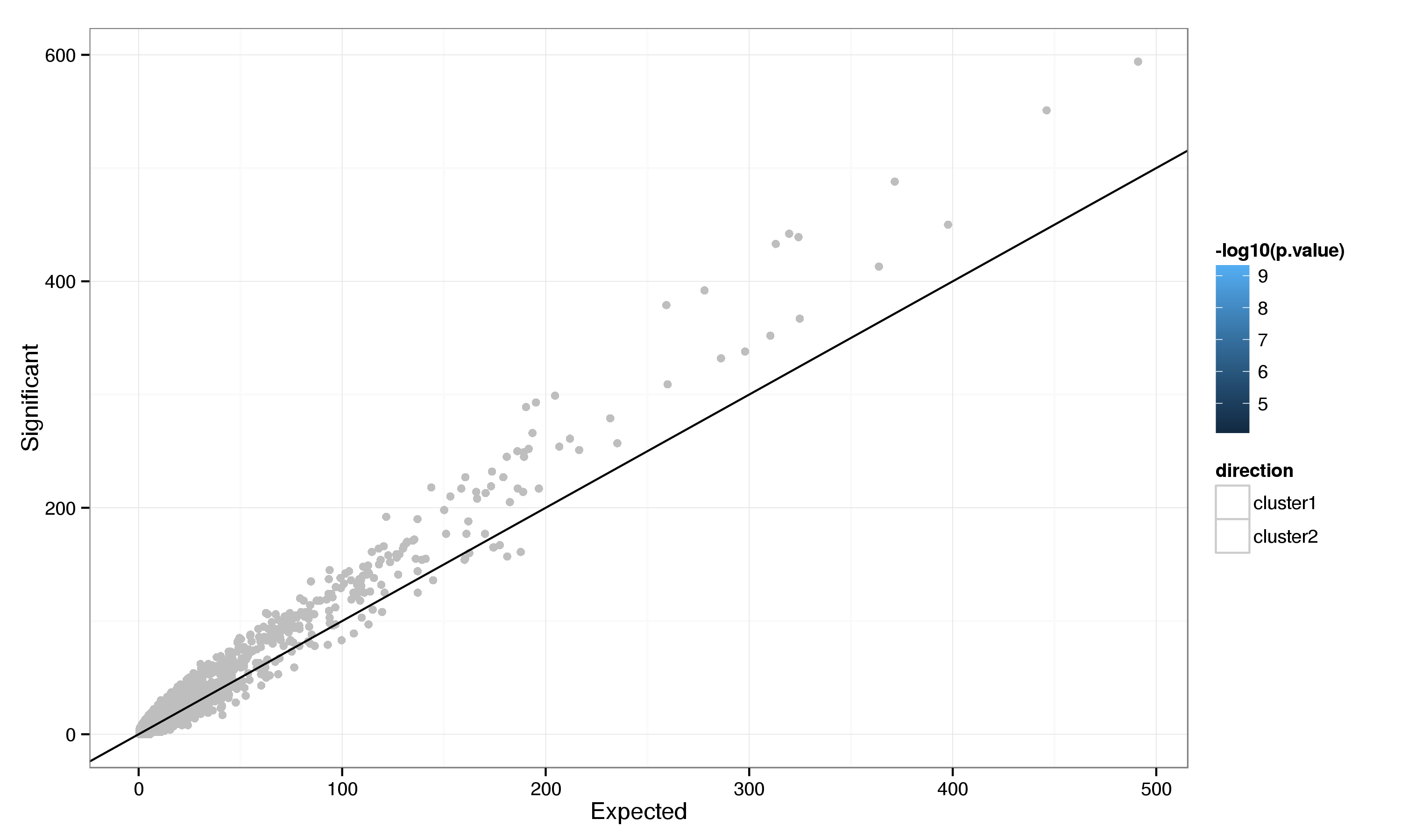
Figure 19: GO category enrichment for genes differentially expressed between PLS clusters.

Appendix

Custom functions used

reshapeData <- function(data, value) {
    ans <- reshape2::melt(data, id.vars = "probe", value.name = value, variable.name = "sample")
    splitLabel <- strsplit(as.character(ans$sample), "_", fixed = TRUE)
    ans$sample <- sapply(splitLabel, "[", 1)
    ans$treatment <- sapply(splitLabel, function(x) x[length(x)])
    as.tbl(ans[c("sample", "treatment", "probe", value)])
}

ibsClust <- function(genome, ...) {
    dst <- spread(dplyr::select(genome, IID1, IID2, DST), IID2, DST)
    size <- nrow(dst) + 1
    labels <- c(as.character(dst$IID1[1]), names(dst)[-1])
    dst <- t(1 - as.matrix(dst[-1]))
    dst <- dst[!is.na(dst)]
    attr(dst, "Size") <- size
    attr(dst, "Labels") <- labels
    attr(dst, "Diag") <- FALSE
    attr(dst, "Upper") <- FALSE
    class(dst) <- "dist"
    
    hclust(dst, ...)
}

pcaClusterPlot <- function(data, i, j, fillColour, legend = TRUE) {
    data <- data[, c("sample", paste0("PC", i), paste0("PC", j), "Sentrix_ID", 
        "cluster")]
    names(data) <- c("sample", "x", "y", "Sentrix_ID", "cluster")
    clusters <- by(data, data$cluster, function(x) x)
    fig <- ggplot(data, aes(x = x, y = y))
    for (cl in clusters) {
        ch <- chull(cl$x, cl$y)
        fig <- fig + geom_polygon(data = cl[ch, ], fill = fillColour[cl$cluster[1]], 
            alpha = 0.7)
    }
    fig <- fig + geom_point(aes(colour = as.character(Sentrix_ID)), size = 3) + 
        theme_bw() + scale_colour_discrete("BeadChip") + xlab(paste0("PC", i)) + 
        ylab(paste0("PC", j))
    if (!legend) 
        fig <- fig + theme(legend.position = "none")
    fig
}

adjustLabel <- function(x, y, centre) {
    just <- c(h = 0, v = 0)
    if (x < centre[1]) {
        just["h"] <- just["h"] + 0.9
    }
    if (y < centre[2]) {
        just["v"] <- just["v"] + 1
    }
    just
}

countBlocks <- function(geno, pval, pcut = 0.05, rcut = 0.8) {
    count <- 0
    selected <- which(pval < pcut)
    if (length(selected)) {
        if (length(selected) == 1) {
            count <- 1
        } else {
            if (names(pval)[1] %in% colnames(geno)) 
                geno <- geno[, names(pval)[selected]] else geno <- t(geno[names(pval)[selected], ])
            r2 <- cor(geno, use = "pairwise", method = "spearman")^2
            remain <- 1:ncol(r2)
            while (length(remain)) {
                i <- remain[1]
                count <- count + 1
                remain <- intersect(which(r2[i, ] < rcut), remain)
            }
        }
    }
    count
}

## Create a scatter plot with one panel per group (by default BeadChip) Data
## points (by default samples in PC space) are assumed to be from a bivariate
## t distribution. Confidence ellipses are drawn based on this (at a 95%
## level by default) and points outside these ellipses are marked as
## outliers.
outlierPlot <- function(data, x = "PC1", y = "PC2", group = "Sentrix_ID", shape = "Treatment", 
    id = "Cell Line", level = 0.95, ...) {
    ellipses <- by(data[, c(x, y)], data[[group]], function(d) tryCatch(car::dataEllipse(as.matrix(d), 
        levels = level, draw = FALSE, robust = TRUE), error = function(e) cbind(NA, 
        NA)))
    data[[group]] <- as.character(data[[group]])
    
    names(data)[which(names(data) == x)] <- make.names(x)
    x <- make.names(x)
    names(data)[which(names(data) == y)] <- make.names(y)
    y <- make.names(y)
    names(data)[which(names(data) == group)] <- make.names(group)
    group <- make.names(group)
    names(data)[which(names(data) == shape)] <- make.names(shape)
    shape <- make.names(shape)
    names(data)[which(names(data) == id)] <- make.names(id)
    id <- make.names(id)
    
    data$outlier <- logical(nrow(data))
    for (i in 1:nrow(data)) {
        data$outlier[i] <- !sp::point.in.polygon(data[i, x], data[i, y], ellipses[[as.character(data[i, 
            group])]][, 1], ellipses[[as.character(data[i, group])]][, 2])
    }
    data$colour <- as.character(data[[group]])
    data$colour[data$outlier] <- NA
    centre <- by(data[, c(x, y)], data[[group]], colMeans)
    data$h <- if (!is.null(list(...)$hjust)) 
        list(...)$hjust else 0
    data$v <- if (!is.null(list(...)$vjust)) 
        list(...)$vjust else 0
    labelJust <- mapply(function(x, y, g, c) adjustLabel(x, y, c[[g]]), data[[x]], 
        data[[y]], data[[group]], MoreArgs = list(centre))
    data$h <- ifelse(labelJust["h", ] > 0, -data$h, data$h)
    data$h <- data$h + labelJust["h", ]
    data$v <- ifelse(labelJust["v", ] > 0, -data$v, data$v)
    data$v <- data$v + labelJust["v", ]
    ggplot(data, aes_string(x = x, y = y, colour = "colour")) + geom_point(aes_string(shape = shape), 
        size = 3) + stat_ellipse(level = level) + facet_wrap(eval(parse(text = paste("~", 
        group))), ncol = 3) + geom_text(data = dplyr::filter(data, outlier), 
        aes_string(label = id, hjust = "h", vjust = "v"), size = 4) + theme_bw() + 
        scale_colour_discrete(guide = "none")
}

plsPlot <- function(plsComp, genotype, groups = "treatment", type = c("present", 
    "genotype")) {
    type <- match.arg(type)
    treatGrp <- by(dplyr::select(plsComp, t1, t2), plsComp[groups], colMeans)
    grps <- do.call(expand.grid, dimnames(treatGrp))
    grps <- dplyr::filter(grps, !sapply(treatGrp, is.null))
    names(grps) <- groups
    treatAvg <- cbind(do.call(rbind, treatGrp), grps)
    if (length(groups) > 1) 
        treatAvg$sample <- treatAvg[[groups[2]]] else treatAvg$sample <- "avg"
    
    if (!missing(genotype)) {
        if (type == "present") {
            plsComp[[genotype]] <- pmin(plsComp[[genotype]], 1)
        }
        plsComp[[genotype]] <- as.factor(plsComp[[genotype]])
        grpMean <- by(dplyr::select(plsComp, t1, t2), c(plsComp[genotype], plsComp[groups]), 
            colMeans)
        grps <- do.call(expand.grid, dimnames(grpMean))
        grps <- dplyr::filter(grps, !sapply(grpMean, is.null))
        names(grps) <- c(genotype, groups)
        genoAvg <- cbind(do.call(rbind, grpMean), grps)
        if (length(groups) > 1) {
            genoAvg$sample <- paste(genoAvg[[genotype]], genoAvg[[groups[2]]], 
                sep = "_")
        } else {
            genoAvg$sample <- genoAvg[[genotype]]
        }
    }
    
    if (length(groups) > 1) {
        fig <- ggplot(plsComp, aes_string(x = "t1", y = "t2", group = "sample", 
            shape = groups[2]))
    } else {
        fig <- ggplot(plsComp, aes_string(x = "t1", y = "t2", group = "sample"))
    }
    if (missing(genotype)) {
        fig <- fig + geom_point(data = treatAvg, aes_string(colour = groups[1]), 
            size = 5)
    } else {
        fig <- fig + geom_point(data = treatAvg, size = 5, colour = "black")
        fig <- fig + geom_point(data = genoAvg, aes_string(colour = genotype), 
            size = 5)
        fig <- fig + geom_line(data = genoAvg, aes_string(colour = genotype), 
            line.width = 2, arrow = grid::arrow(type = "closed", length = grid::unit(0.15, 
                "inches"), angle = 20))
    }
    fig <- fig + geom_line(data = treatAvg, colour = "black", line.width = 2, 
        arrow = grid::arrow(type = "closed", length = grid::unit(0.15, "inches"), 
            angle = 20))
    if (missing(genotype)) {
        fig <- fig + geom_point(aes_string(colour = groups[1]), size = 3, alpha = 0.6)
        fig <- fig + scale_colour_manual(values = c(Basal = "blue", Stim = "red"))
    } else {
        fig <- fig + geom_point(aes_string(colour = genotype), size = 3, alpha = 0.6)
        fig <- fig + scale_colour_manual(values = c(`0` = "#3E79F7", `1` = "#FA2AA4", 
            `2` = "#FFB72B"))
    }
    fig <- fig + geom_line(colour = "grey", alpha = 0.6, arrow = grid::arrow(type = "closed", 
        length = grid::unit(0.15, "inches"), angle = 20))
    
    fig <- fig + theme_bw() + xlab("Component 1") + ylab("Component 2")
    fig
}

volcanoPlot <- function(limmaTable, fcCut, fdrCut, fcCut2 = log2(2)) {
    fcScale <- max(-log10(limmaTable$adj.P.Val))/max(abs(limmaTable$logFC))
    limmaExtreme <- dplyr::filter(limmaTable, abs(logFC) > fcCut & adj.P.Val < 
        fdrCut)
    limmaExtreme <- mutate(limmaExtreme, distance = (fcScale * logFC)^2 + log10(adj.P.Val)^2)
    limmaExtreme <- limmaExtreme[order(limmaExtreme$distance, decreasing = TRUE), 
        ]
    ggplot(limmaTable, aes(x = logFC, y = -log10(adj.P.Val))) + stat_density2d(data = dplyr::filter(limmaTable, 
        abs(logFC) <= fcCut | adj.P.Val >= fdrCut), geom = "tile", aes(fill = ..density..^0.1), 
        contour = FALSE) + geom_point(data = limmaExtreme, size = 1.5, aes(colour = distance)) + 
        geom_text(data = dplyr::filter(limmaExtreme, distance > (2 * fcScale)^2 & 
            logFC >= fcCut2), aes(label = SymbolReannotated), vjust = 0, hjust = 0, 
            angle = 30) + geom_text(data = dplyr::filter(limmaExtreme, distance > 
        (2 * fcScale)^2 & logFC <= -fcCut2), aes(label = SymbolReannotated), 
        vjust = 0, hjust = 1, angle = 330) + geom_line(data = data.frame(x = c(-Inf, 
        -fcCut), y = c(-log10(fdrCut), -log10(fdrCut))), aes(x = x, y = y), 
        linetype = "dotted") + geom_line(data = data.frame(x = c(fcCut, Inf), 
        y = c(-log10(fdrCut), -log10(fdrCut))), aes(x = x, y = y), linetype = "dotted") + 
        geom_line(data = data.frame(x = c(fcCut, fcCut), y = c(-log10(fdrCut), 
            Inf)), aes(x = x, y = y), linetype = "dotted") + geom_line(data = data.frame(x = c(-fcCut, 
        -fcCut), y = c(-log10(fdrCut), Inf)), aes(x = x, y = y), linetype = "dotted") + 
        scale_fill_gradientn(colours = colorRampPalette(c("white", blues9))(256), 
            breaks = NULL) + scale_colour_gradientn(colours = colorRampPalette(c("yellow", 
        "red"))(256), guide = "none") + theme_bw() + xlab("log2(fold change)") + 
        ylab("-log10(FDR)") + expand_limits(x = c(min(limmaTable$logFC) - 0.25, 
        max(limmaTable$logFC) + 0.25), y = max(-log10(limmaTable$adj.P.Val)) + 
        2)
}
# Multiple plot function ggplot objects can be passed in ..., or to plotlist
# (as a list of ggplot objects) - cols: Number of columns in layout -
# layout: A matrix specifying the layout. If present, 'cols' is ignored.  If
# the layout is something like matrix(c(1,2,3,3), nrow=2, byrow=TRUE), then
# plot 1 will go in the upper left, 2 will go in the upper right, and 3 will
# go all the way across the bottom.  author: Winston Chang ()
multiplot <- function(..., plotlist = NULL, file, cols = 1, layout = NULL) {
    library(grid)
    
    # Make a list from the ... arguments and plotlist
    plots <- c(list(...), plotlist)
    
    numPlots = length(plots)
    
    # If layout is NULL, then use 'cols' to determine layout
    if (is.null(layout)) {
        # Make the panel ncol: Number of columns of plots nrow: Number of rows
        # needed, calculated from # of cols
        layout <- matrix(seq(1, cols * ceiling(numPlots/cols)), ncol = cols, 
            nrow = ceiling(numPlots/cols))
    }
    
    if (numPlots == 1) {
        print(plots[[1]])
        
    } else {
        # Set up the page
        grid.newpage()
        pushViewport(viewport(layout = grid.layout(nrow(layout), ncol(layout))))
        
        # Make each plot, in the correct location
        for (i in 1:numPlots) {
            # Get the i,j matrix positions of the regions that contain this subplot
            matchidx <- as.data.frame(which(layout == i, arr.ind = TRUE))
            
            print(plots[[i]], vp = viewport(layout.pos.row = matchidx$row, layout.pos.col = matchidx$col))
        }
    }
}

filterSample <- function(sig, sig.raw, det, excl) {
    sig <- filter(sig, !sample %in% excl)
    sig.raw <- filter(sig.raw, !sample %in% excl)
    det <- filter(det, !sample %in% excl)
    
    list(sig = sig, sig.raw = sig.raw, det = det)
}

updateSampleList <- function(samples, sampleFile) {
    samples <- sub("_.", "", unique(samples))
    sampleInfo <- readr::read_delim(sampleFile, delim = " ", col_names = c("Family", 
        "Individual", "Father", "Mother", "Sex", "Phenotype"))
    keepSamples <- dplyr::filter(dplyr::select(sampleInfo, Family, Individual), 
        Individual %in% samples)
    write.table(keepSamples, file = "tmp/sample.lst", quote = FALSE, col.names = FALSE, 
        row.names = FALSE)
    invisible(keepSamples)
}

formatQTL <- function(me, limmaTable) {
    eQTL <- me$all$eqtls
    eQTL <- dplyr::left_join(eQTL, dplyr::select(limmaTable, NuID, SymbolReannotated, 
        AveExpr, logFC), by = c(gene = "NuID"))
    eQTL <- dplyr::select(eQTL, snps, SymbolReannotated, gene, beta:FDR, AveExpr, 
        logFC)
    eQTL <- dplyr::rename(eQTL, SNP = snps, Gene = SymbolReannotated, NuID = gene)
    eQTL
}

promoterScan <- function(seqs, pwms, group) {
    res <- motifEnrichment(seqs, pwms)
    report <- lapply(1:length(seqs), function(x, i) sequenceReport(x, i)@d, 
        x = res)
    report <- do.call(rbind, report)
    cbind(report, EntrezReannotated = names(seqs), expr = group)
}

plsLimma <- function(data, cluster) {
    design <- model.matrix(~0 + cluster)
    contrasts <- makeContrasts(cluster3 - cluster1, cluster3 - cluster2, cluster1 - 
        cluster2, levels = design)
    clusterFit <- lmFit(data, design)
    clusterFit2 <- contrasts.fit(clusterFit, contrasts)
    clusterFit2 <- eBayes(clusterFit2)
    
    clust3_1Table <- topTable(clusterFit2, coef = 1, n = dim(clusterFit2)[1], 
        adjust = "BH")
    clust3_2Table <- topTable(clusterFit2, coef = 2, n = dim(clusterFit2)[1], 
        adjust = "BH")
    clust1_2Table <- topTable(clusterFit2, coef = 3, n = dim(clusterFit2)[1], 
        adjust = "BH")
    
    clust3_1Table <- cbind(ArrayAddress = rownames(clust3_1Table), clust3_1Table)
    clust3_1Table <- inner_join(dplyr::select(annot, ArrayAddress, NuID, SymbolReannotated, 
        EntrezReannotated, GenomicLocation), clust3_1Table)
    clust3_1Table <- clust3_1Table[order(clust3_1Table$P.Value), ]
    
    clust3_2Table <- cbind(ArrayAddress = rownames(clust3_2Table), clust3_2Table)
    clust3_2Table <- inner_join(dplyr::select(annot, ArrayAddress, NuID, SymbolReannotated, 
        EntrezReannotated, GenomicLocation), clust3_2Table)
    clust3_2Table <- clust3_2Table[order(clust3_2Table$P.Value), ]
    
    clust1_2Table <- cbind(ArrayAddress = rownames(clust1_2Table), clust1_2Table)
    clust1_2Table <- inner_join(dplyr::select(annot, ArrayAddress, NuID, SymbolReannotated, 
        EntrezReannotated, GenomicLocation), clust1_2Table)
    clust1_2Table <- clust1_2Table[order(clust1_2Table$P.Value), ]
    list(clust3_1Table = clust3_1Table, clust3_2Table = clust3_2Table, clust1_2Table = clust1_2Table)
}
prep_topGO <- function(limmaTable, fdrCut, fcCut) {
    groupUp <- ifelse(limmaTable$adj.P.Val < fdrCut & limmaTable$logFC > fcCut, 
        1, 0)
    groupDown <- ifelse(limmaTable$adj.P.Val < fdrCut & limmaTable$logFC < -fcCut, 
        1, 0)
    groupAll <- ifelse(limmaTable$adj.P.Val < fdrCut & abs(limmaTable$logFC) > 
        fcCut, 1, 0)
    
    universeUp <- factor(groupUp)
    names(universeUp) <- limmaTable$EntrezReannotated
    universeUp <- universeUp[!is.na(names(universeUp))]
    universeDown <- factor(groupDown)
    names(universeDown) <- limmaTable$EntrezReannotated
    universeDown <- universeDown[!is.na(names(universeDown))]
    universeAll <- factor(groupAll)
    names(universeAll) <- limmaTable$EntrezReannotated
    universeAll <- universeAll[!is.na(names(universeAll))]
    
    tgUp <- new("topGOdata", ontology = "BP", allGenes = universeUp, nodeSize = 10, 
        description = "Genes up-regulated after heat shock", annotationFun = annFUN.org, 
        mapping = "org.Hs.eg.db")
    tgDown <- new("topGOdata", ontology = "BP", allGenes = universeDown, nodeSize = 10, 
        description = "Genes down-regulated after heat shock", annotationFun = annFUN.org, 
        mapping = "org.Hs.eg.db")
    tgAny <- new("topGOdata", ontology = "BP", allGenes = universeAll, nodeSize = 10, 
        description = "Genes differentially expressed in response to heat shock", 
        annotationFun = annFUN.org, mapping = "org.Hs.eg.db")
    
    list(up = tgUp, down = tgDown, any = tgAny)
}

figRef <- local({
    tag <- numeric()
    created <- logical()
    used <- logical()
    function(label, caption, prefix = options("figcap.prefix"), sep = options("figcap.sep"), 
        prefix.highlight = options("figcap.prefix.highlight")) {
        i <- which(names(tag) == label)
        if (length(i) == 0) {
            i <- length(tag) + 1
            tag <<- c(tag, i)
            names(tag)[length(tag)] <<- label
            used <<- c(used, FALSE)
            names(used)[length(used)] <<- label
            created <<- c(created, FALSE)
            names(created)[length(created)] <<- label
        }
        if (!missing(caption)) {
            created[label] <<- TRUE
            paste0(prefix.highlight, prefix, " ", i, sep, prefix.highlight, 
                " ", caption)
        } else {
            used[label] <<- TRUE
            paste(prefix, tag[label])
        }
    }
})

tabRef <- local({
    tag <- numeric()
    created <- logical()
    used <- logical()
    function(label, caption, prefix = options("tabcap.prefix"), sep = options("tabcap.sep"), 
        prefix.highlight = options("tabcap.prefix.highlight")) {
        i <- which(names(tag) == label)
        if (length(i) == 0) {
            i <- length(tag) + 1
            tag <<- c(tag, i)
            names(tag)[length(tag)] <<- label
            used <<- c(used, FALSE)
            names(used)[length(used)] <<- label
            created <<- c(created, FALSE)
            names(created)[length(created)] <<- label
        }
        if (!missing(caption)) {
            created[label] <<- TRUE
            paste0(prefix.highlight, prefix, " ", i, sep, prefix.highlight, 
                " ", caption)
        } else {
            used[label] <<- TRUE
            paste(prefix, tag[label])
        }
    }
})

Session Info

R version 3.2.1 (2015-06-18) Platform: x86_64-pc-linux-gnu (64-bit) Running under: Debian GNU/Linux stretch/sid

locale: [1] LC_CTYPE=en_US.UTF-8 LC_NUMERIC=C
[3] LC_TIME=en_US.UTF-8 LC_COLLATE=en_US.UTF-8
[5] LC_MONETARY=en_US.UTF-8 LC_MESSAGES=en_US.UTF-8
[7] LC_PAPER=en_US.UTF-8 LC_NAME=C
[9] LC_ADDRESS=C LC_TELEPHONE=C
[11] LC_MEASUREMENT=en_US.UTF-8 LC_IDENTIFICATION=C

attached base packages: [1] grid stats4 parallel methods stats graphics grDevices [8] utils datasets base

other attached packages: [1] PWMEnrich.Hsapiens.background_4.2.0
[2] PWMEnrich_4.4.0
[3] biomaRt_2.24.0
[4] RISmed_2.1.5
[5] MultiPhen_2.0.1
[6] meta_4.3-0
[7] epitools_0.5-7
[8] abind_1.4-3
[9] plsdepot_0.1.17
[10] MatrixEQTL_2.1.1
[11] plink2R_1.0
[12] RcppEigen_0.3.2.5.0
[13] Rcpp_0.12.0
[14] TxDb.Hsapiens.UCSC.hg19.knownGene_3.1.2 [15] GenomicFeatures_1.20.1
[16] BSgenome.Hsapiens.UCSC.hg19_1.4.0
[17] SNPlocs.Hsapiens.dbSNP142.GRCh37_0.99.5 [18] BSgenome_1.36.2
[19] rtracklayer_1.28.6
[20] Biostrings_2.36.1
[21] XVector_0.8.0
[22] GenomicRanges_1.20.5
[23] topGO_2.20.0
[24] SparseM_1.6
[25] GO.db_3.1.2
[26] graph_1.46.0
[27] ggdendro_0.1-15
[28] reshape2_1.4.1
[29] pander_0.5.2
[30] illuminaHumanv3.db_1.26.0
[31] org.Hs.eg.db_3.1.2
[32] RSQLite_1.0.0
[33] DBI_0.3.1
[34] AnnotationDbi_1.30.1
[35] GenomeInfoDb_1.4.1
[36] IRanges_2.2.5
[37] S4Vectors_0.6.2
[38] stringr_1.0.0
[39] readr_0.1.1.9000
[40] tidyr_0.2.0
[41] dplyr_0.4.2
[42] ggplot2_1.0.1
[43] RColorBrewer_1.1-2
[44] gplots_2.17.0
[45] sva_3.14.0
[46] genefilter_1.50.0
[47] mgcv_1.8-6
[48] nlme_3.1-121
[49] scatterplot3d_0.3-36
[50] limma_3.24.15
[51] vsn_3.36.0
[52] affy_1.46.1
[53] Biobase_2.28.0
[54] BiocGenerics_0.14.0
[55] gdata_2.17.0
[56] proto_0.3-10
[57] MASS_7.3-42
[58] pushoverr_0.1.4
[59] knitrBootstrap_1.0.0
[60] knitr_1.11
[61] rmarkdown_0.7
[62] BiocInstaller_1.18.4

loaded via a namespace (and not attached): [1] minqa_1.2.4 colorspace_1.2-6
[3] evd_2.3-0 markdown_0.7.7
[5] futile.logger_1.4.1 mice_2.22
[7] affyio_1.36.0 codetools_0.2-11
[9] splines_3.2.1 R.methodsS3_1.7.0
[11] nloptr_1.0.4 Rsamtools_1.20.4
[13] seqLogo_1.34.0 pbkrtest_0.4-2
[15] annotate_1.46.1 R.oo_1.19.0
[17] httr_1.0.0 assertthat_0.1
[19] Matrix_1.2-2 lazyeval_0.1.10
[21] formatR_1.2 quantreg_5.11
[23] htmltools_0.2.6 tools_3.2.1
[25] gtable_0.1.2 preprocessCore_1.30.0
[27] lme4_1.1-8 gtools_3.5.0
[29] XML_3.98-1.3 zlibbioc_1.14.0
[31] scales_0.2.5 lambda.r_1.1.7
[33] HardyWeinberg_1.5.5 yaml_2.1.13
[35] rpart_4.1-10 stringi_0.5-5
[37] randomForest_4.6-10 caTools_1.17.1
[39] BiocParallel_1.2.9 bitops_1.0-6
[41] evaluate_0.7.2 lattice_0.20-31
[43] GenomicAlignments_1.4.1 labeling_0.3
[45] plyr_1.8.3 magrittr_1.5
[47] R6_2.1.0 sp_1.1-1
[49] survival_2.38-3 RCurl_1.95-4.7
[51] nnet_7.3-10 car_2.0-25
[53] futile.options_1.0.0 KernSmooth_2.23-15
[55] digest_0.6.8 xtable_1.7-4
[57] R.utils_2.1.0 munsell_0.4.2

References

Alexa, Adrian, and Jorg Rahnenfuhrer. 2010. TopGO: TopGO: Enrichment Analysis for Gene Ontology.

Barbosa-Morais, Nuno L., Mark J. Dunning, Shamith A. Samarajiwa, Jeremy F. J. Darot, Matthew E. Ritchie, Andy G. Lynch, and Simon Tavaré. 2010. “A Re-Annotation Pipeline for Illumina BeadArrays: Improving the Interpretation of Gene Expression Data.” Nucleic Acids Research 38 (3): e17. doi:10.1093/nar/gkp942.

Carlson, Marc. 2015. TxDb.Hsapiens.UCSC.hg19.knownGene: Annotation Package for TxDb Object(s).

Chang, Christopher, Carson Chow, Laurent Tellier, Shashaank Vattikuti, Shaun Purcell, and James Lee. 2015. “Second-Generation PLINK: Rising to the Challenge of Larger and Richer Datasets.” GigaScience 4 (1): 7. doi:10.1186/s13742-015-0047-8.

Gibbs, Richard et al. 2010. “The International HapMap Project.” Nature 426: 789–96.

Huber, Wolfgang, Anja von Heydebreck, Holger Sueltmann, Annemarie Poustka, and Martin Vingron. 2002. “Variance Stabilization Applied to Microarray Data Calibration and to the Quantification of Differential Expression.” Bioinformatics 18 Suppl. 1: S96–S104.

Johnson, W. Evan, Cheng Li, and Ariel Rabinovic. 2007. “Adjusting Batch Effects in Microarray Expression Data Using Empirical Bayes Methods.” Biostatistics 8 (1): 118–27. doi:10.1093/biostatistics/kxj037.

Kee, C., K. Y. Cheong, K. Pham, G. W. Waterer, and S. E. L. Temple. 2008. “Genetic Variation in Heat Shock Protein 70 Is Associated with Septic Shock: Narrowing the Association to a Specific Haplotype.” International Journal of Immunogenetics 35 (6). Blackwell Publishing Ltd: 465–73. doi:10.1111/j.1744-313X.2008.00812.x.

Leek, Jeffrey T., W. Evan Johnson, Hilary S. Parker, Elana J. Fertig, Andrew E. Jaffe, and John D. Storey. 2015. Sva: Surrogate Variable Analysis.

Martin, Annalise M., David Nolan, Silvana Gaudieri, Coral Ann Almeida, Richard Nolan, Ian James, Filipa Carvalho, et al. 2004. “Predisposition to Abacavir Hypersensitivity Conferred by HLA-B*5701 and a Haplotypic Hsp70-Hom Variant.” Proceedings of the National Academy of Sciences 101 (12): 4180–85. doi:10.1073/pnas.0307067101.

O’Reilly, Clive J. AND Pomyen, Paul F. AND Hoggart. 2012. “MultiPhen: Joint Model of Multiple Phenotypes Can Increase Discovery in GWAS.” PLoS ONE 7 (5). Public Library of Science: e34861. doi:10.1371/journal.pone.0034861.

Pachkov, Mikhail, Ionas Erb, Nacho Molina, and Erik van Nimwegen. 2007. “SwissRegulon: A Database of Genome-Wide Annotations of Regulatory Sites.” Nucleic Acids Research 35 (suppl 1): D127–31. doi:10.1093/nar/gkl857.

Pagès, Hervé. 2014. SNPlocs.Hsapiens.dbSNP142.GRCh37: SNP Locations for Homo Sapiens (DbSNP Build 142).

Richter, Klaus, Martin Haslbeck, and Johannes Buchner. 2010. “The Heat Shock Response: Life on the Verge of Death.” Molecular Cell 40 (2). Elsevier: 253–66. doi:10.1016/j.molcel.2010.10.006.

Ritchie, Matthew E, Belinda Phipson, Di Wu, Yifang Hu, Charity W Law, Wei Shi, and Gordon K Smyth. 2015. “limma Powers Differential Expression Analyses for RNA-Sequencing and Microarray Studies.” Nucleic Acids Research 43: doi: 10.1093/nar/gkv007.

Ritossa, Ferruccio. 1962. “A New Puffing Pattern Induced by Temperature Shock and DNP in Drosophila.” Experientia 18: 571–73.

Sfar, Sana, Hamadi Saad, Faouzi Mosbah, and Lotfi Chouchane. 2010. “Synergistic Effect and VEGF/HSP70-Hom Haplotype Analysis: Relationship to Prostate Cancer Risk and Clinical Outcome.” Human Immunology 71 (4): 377–82. doi:http://dx.doi.org/10.1016/j.humimm.2010.01.017.

Stojnic, Robert, and Diego Diez. 2014. PWMEnrich: PWM Enrichment Analysis.

Vihervaara, Anniina, Christian Sergelius, Jenni Vasara, Malin A. H. Blom, Alexandra N. Elsing, Pia Roos-Mattjus, and Lea Sistonen. 2013. “Transcriptional Response to Stress in the Dynamic Chromatin Environment of Cycling and Mitotic Cells.” Proceedings of the National Academy of Sciences 110 (36): E3388–97. doi:10.1073/pnas.1305275110.

Styled with knitrBootstrap