Introduction to eQTL analysis

Peter Humburg

Overview

Hands-on : Setup
What are eQTL?
Detecting eQTL – A simple model
Hands-on : Simple linear regression
Detecting eQTL – Not that simple
Hands-on : Covariates
Covariates – Choose wisely
If only we knew – Covariates for real data
Hands-on : Dealing with real data
Large scale eQTL analysis
Hands-on : Scaling it up
Interpreting results
Summary

Hands-on : Setup

Docker image

Make sure you have the latest version of the docker image.

docker pull humburg/eqtl-intro

Directory structure

Create a working directory for this course. (eqtl_course)
Within that directory, create two sub-directories
- genotypes
- analysis
Mac: create directories under /Users/
Windows: create directories under C:\Users\

Additional data

The docker image contains most of the data. Further genotyping data is available from

ftp://galahad.well.ox.ac.uk

Username: eqtl_course

Download the data and save it into genotypes

Start the RStudio server

Windows :

docker run -p 8787:8787 
  -v /c/Users/user/eqtl_course/genotpes:/data/genotypes
  humburg/eqtl-intro

IP address of the server usually is 192.168.59.103.

Use boot2docker ip to check if necessary.

Start the RStudio server

Mac :

docker run -p 8787:8787 
   -v /Users/user/eqtl_course/genotpes:/data/genotypes 
   humburg/eqtl-intro

IP address of the server usually is 192.168.59.103.

Use boot2docker ip to check if necessary.

Start the RStudio server

Linux :

docker run -p 8787:8787 
  -v /home/user/eqtl_course/genotpes:/data/genotypes
  -e USER=$USER  -e USERID = $UID 
  humburg/eqtl-intro

IP address of the server usually is 127.0.0.1 (or localhost).

Using RStudio

Access the RStudio interface at http://yourip:8787.

* Username: rstudio
* Password: rstudio

Useful resources

RStudio cheat sheets

What are eQTL?

Quantitative trait loci

QTL are regions of the genome associated with quantitative traits

height
BMI
lung capacity
…

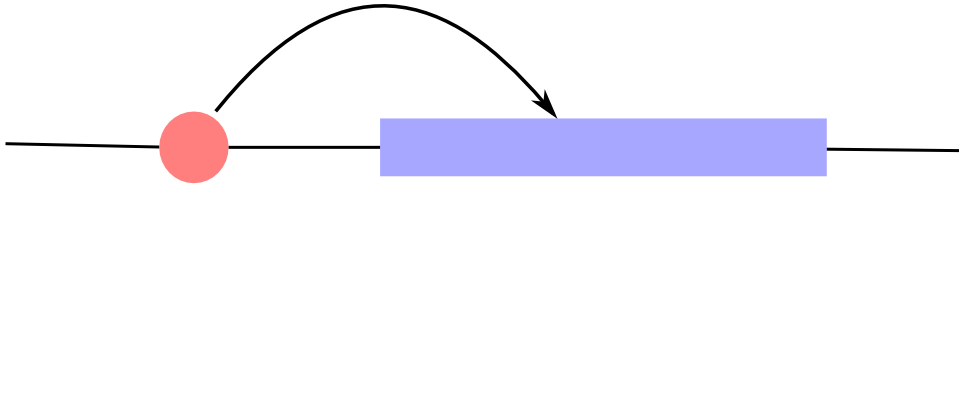
Expression quantitative trait loci

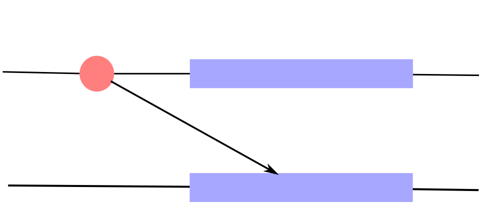
If the trait of interest is the expression of a gene, we talk about eQTL.

Associations can be local (cis)
or distant (trans)

Expression quantitative trait loci

If the trait of interest is the expression of a gene, we talk about eQTL.

Associations can be local (cis)
or distant (trans)

Expression quantitative trait loci

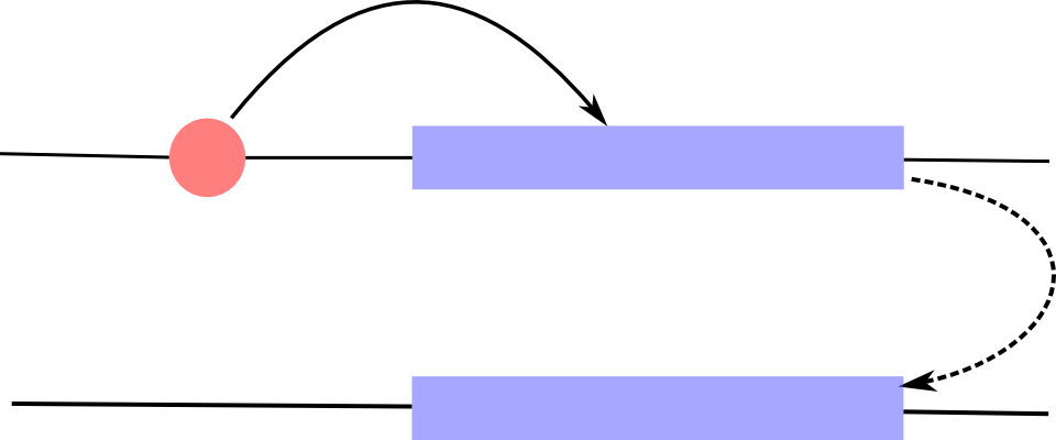
If the trait of interest is the expression of a gene, we talk about eQTL.

Associations can be local (cis)
or distant (trans)

Detecting eQTL – A simple model

How do we know whether a locus is associated with the expression of a gene?

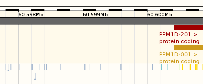
Any given locus contains multiple SNPs.
Can determine genotypes for these SNPs in a (large) number of individuals.
Measure gene expression for genes of interest.
Assess the evidence that expression varies with genotype.

How do we know whether a locus is associated with the expression of a gene?

sample	snp_1	snp_2	snp_3	…
sample 1	AA	AA	AB	…
sample 2	AB	AB	AA	…
sample 3	AB	BB	AB	…
…	…	…	…	…

Any given locus contains multiple SNPs.
Can determine genotypes for these SNPs in a (large) number of individuals.
Measure gene expression for genes of interest.
Assess the evidence that expression varies with genotype.

How do we know whether a locus is associated with the expression of a gene?

sample	gene_1	gene_2	gene_3	…
sample 1	7.3	12.8	6.5	…
sample 2	10.9	9.6	8.8	…
sample 3	9.5	10.7	15.1	…
…	…	…	…	…

Any given locus contains multiple SNPs.
Can determine genotypes for these SNPs in a (large) number of individuals.
Measure gene expression for genes of interest.
Assess the evidence that expression varies with genotype.

How do we know whether a locus is associated with the expression of a gene?

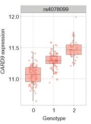
Any given locus contains multiple SNPs.
Can determine genotypes for these SNPs in a (large) number of individuals.
Measure gene expression for genes of interest.
Assess the evidence that expression varies with genotype.

Linear additive model

Different alleles of a SNP may exhibit a dosage effect.

Using the AA genotype as baseline, each copy of the B allele changes expression by a fixed amount.
Implies a linear relationship between the mean gene expression and the number of B alleles.
Estimating the change in expression due to the B allele to quantify the SNP’s contribution to gene expression.

Linear regression

\[Y = \beta_0 + \beta X + \varepsilon\]

Y: Response variable (here: vector of expression values for gene of interest).
X: Explanatory variable (here: vector of genotypes (coded as 0, 1, 2) for the SNP under consideration).

Linear regression

\[Y = \beta_0 + \beta X + \varepsilon\]

\(\beta_0\): Intercept (here: mean expression for AA genotype).
\(\beta\): Regression coefficient; the effect of X on the mean of Y (here: change in mean gene expression for each copy of the B allele).
\(\varepsilon\): Residuals; the difference between observed values of \(Y\) and the estimated mean of \(Y|X\)

Linear regression – Assumptions

Residuals are

independent
normally distributed with mean 0 and constant variance

It is implied that

There is a linear relationship between \(X\) and \(Y\).
Values of \(Y\) for each value of \(X\) are normally distributed.
There is only one source of variation not explained by \(X\).

Linear regression – Robustness

Independence of residuals

Lack of independence can produce misleading results.

What could cause this?

Linear regression – Robustness

Constant variance of residuals (homoskedacity)

Violation of this assumption will lead to incorrect p-values and confidence intervals.

Linear regression – Robustness

Normality

Estimates and their confidence intervals and p-values are fairly robust.
But beware of long tailed distributions.
Prediction can become problematic (but we are not interested in that here).

Linear regression – Robustness

Linearity

If the true relationship between \(Y\) and \(X\) is non-linear conclusions may be misleading.

When might this occur with eQTL data?

Linear regression – Robustness

Linearity

If the true relationship between \(Y\) and \(X\) is non-linear conclusions may be misleading.

When might this occur with eQTL data?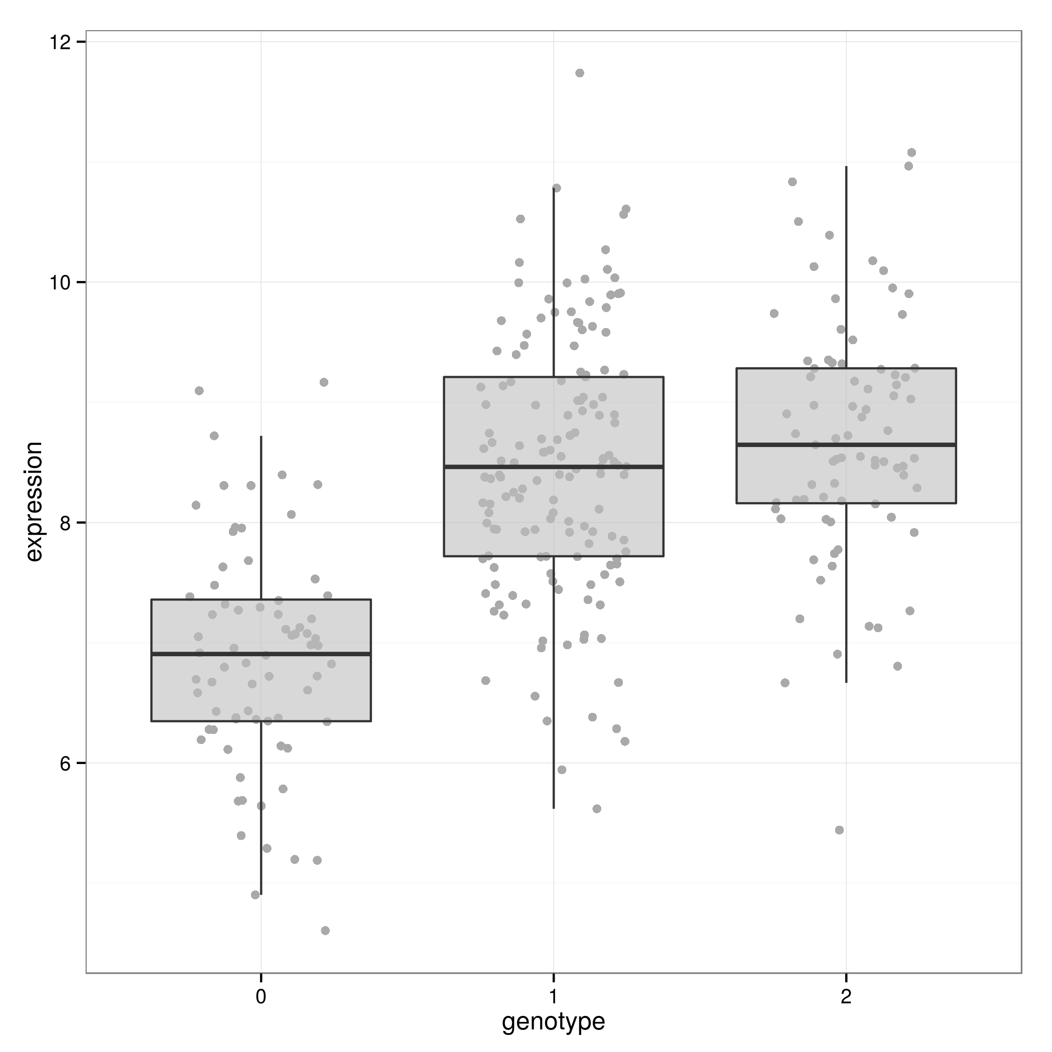

Hands-on : Simple linear regression

Data

Genotypes: /data/simulated/sim_genotypes.tab
Gene expression: /data/simulated/sim_expression1.tab

Warm-up

Load the data into R.
How is the data formatted?
Determine minor allele frequencies.

geno <- readr::read_tsv("/data/simulated/sim_genotypes.tab")
expr <- readr::read_tsv("/data/simulated/sim_expression1.tab")

maf <- colMeans(geno[-1])/2

Plotting the data

Choose a SNP/gene pair (snp_1 / gene_1, snp_2 / gene_2, …)
Create a plot showing gene expression by genotype for this pair.

Assign SNP/gene pairs to participants to ensure each is handled at least once.

library(ggplot2)
genoLong <- tidyr::gather(geno, snp, genotype, -sample)
exprLong <- tidyr::gather(expr, gene, expression, -sample)
dataLong <- cbind(genoLong, exprLong["expression"])
dataLong$genotype <- as.factor(dataLong$genotype) 
ggplot(dataLong, aes(genotype, expression)) +
        geom_jitter(colour="darkgrey", 
                position=position_jitter(width=0.25)) +
        geom_boxplot(outlier.size=0, alpha=0.6, fill="grey") + 
        facet_wrap(~snp) + theme_bw()

Fitting a simple linear regression

Fit a simple linear regression for the SNP/gene pair of your choice.
Compute the 95% confidence interval for the genotype effect.

Collect results from participants into a file and load into R.

Code fit all models is below.

fit <- mapply(function(e, g) lm(e ~ g), 
        expr[-1], geno[-1], SIMPLIFY=FALSE)
betaHat <- sapply(fit, coef)[2,]

ci <- sapply(fit, confint, "g")
rownames(ci) <- c("lower", "upper")

Examining the results

Create diagnostic plots.
Plot estimated genotype effects by minor allele frequency.

Display R’s build-in diagnostics by plotting the fit object.

The true SNP effect is 1.5

estimates <- data.frame(estimate=betaHat, t(ci), maf=maf)
fig <- ggplot(estimates, aes(x=maf)) +  
        geom_hline(yintercept=0, linetype="longdash") + 
        geom_errorbar(aes(ymin=lower, ymax=upper)) +
        geom_point(aes(y=estimate))  + theme_bw()
fig <- fig + geom_hline(yintercept=1.5)

Interlude: p-values

After estimating model coefficients we can test them for departure from 0.
We are interested in identifying SNPs with non-zero coefficients.
The strength of the evidence that the true coefficient is non-zero is often gauged by the resulting p-value.
How should p-values be interpreted?

Detecting eQTL – Not that simple

Additional sources of variation

Gene expression is subject to many sources of variation.
A model with a single SNP as explanatory variable is unlikely to be sufficient.

Use multiple regression to obtain better estimates of SNP effects.

Multiple regression

\[Y = \beta_0 + \sum_{i=1}^n \beta_i X_i + \varepsilon\]

Similar to simple linear regression but incorporates multiple explanatory variables.
\(\beta_i\) are interpreted as “change of \(Y\) due to a unit change in \(X_i\) when all other explanatory variables are held constant”.

Explanatory variables are assumed to be uncorrelated with each other.

Hands-on : Covariates

Data

Genotypes: /data/simulated/sim_genotypes.tab
Gene expression: /data/simulated/sim_expression2.tab
Covariates: /data/simulated/sim_covariates.tab

Plotting the data

Create a plot of gene expression by genotype for you SNP/gene pair of choice.

How does this compare to the plot from the previous exercise.

library(ggplot2)
genoLong <- tidyr::gather(geno, snp, genotype, -sample)
exprLong <- tidyr::gather(expr, gene, expression, -sample)
dataLong <- cbind(genoLong, exprLong["expression"])
dataLong$genotype <- as.factor(dataLong$genotype) 
ggplot(dataLong, aes(genotype, expression)) +
        geom_jitter(colour="darkgrey", 
                position=position_jitter(width=0.25)) +
        geom_boxplot(outlier.size=0, alpha=0.6, fill="grey") + 
        facet_wrap(~snp) + theme_bw()

There is very little evidence of a SNP effect in these plots.

Simple linear regression

Repeat the simple linear regession analysis with these data.

Fit a model for one of the SNP/gene pairs
Create diagnostic plots
Compute the confidence interval for the coefficient

How does this compare to the result from the previous analysis?

simpleFit <- mapply(function(e, g) lm(e ~ g), 
        expr[-1], geno[-1], SIMPLIFY=FALSE)
simpleBetaHat <- sapply(simpleFit, coef)[2,]
simpleCI <- sapply(simpleFit, confint, "g")
rownames(simpleCI) <- c("lower", "upper")

Plot all results:

maf <- colMeans(geno[-1])/2
estimates <- data.frame(estimate=simpleBetaHat, t(simpleCI), maf=maf)
ggplot(estimates, aes(x=maf)) + geom_hline(yintercept=1.5) + 
        geom_hline(yintercept=0, linetype="longdash") + 
        geom_errorbar(aes(ymin=lower, ymax=upper)) +
        geom_point(aes(y=estimate))  + theme_bw()

Note that the true SNP coefficient is still 1.5 but estimates are considerably worse.

Multiple linear regression

Use the first five variables contained in the covariates file as covariates in your model.
Create diagnostic plots
Compute the confidence interval for the coefficient

covarFit <- mapply(function(e, g, var) lm(e ~ g + var), 
        expr[-1], geno[-1], 
        MoreArgs=list(as.matrix(covar[2:6])), SIMPLIFY=FALSE)
covarBetaHat <- sapply(covarFit, coef)[2,]
covarCI <- sapply(covarFit, confint, "g")
rownames(covarCI) <- c("lower", "upper")

May also want to try including all 20 variables.

Covariates – Choose wisely

(Multi)-colinearity

If \(X_i\) and \(X_j\) are correlated the estimates of \(\beta_i\) and \(\beta_j\) will be biased. Several issues may occur:

All the variance in \(Y\) due to \(X_i\) and \(X_j\) is wholly attributed to one of the variables (say, \(X_i\)).
- Results in over estimation of \(\beta_i\) and under estimation of \(\beta_j\)
Estimates for both \(\beta_i\) and \(\beta_j\) are too low because all of the variance is explained by the other variable that is held constant.
No sensible interpretation for \(\beta_i\) and \(\beta_j\).
Model fitting may fail.

Dealing with colinearity

Check correlation between explanatory variables.
Check variance inflation factor (VIF).
Choose only one from each group of correlated variables.

Only really need to worry about variables of interest for downstream analysis.

If only we knew – Covariates for real data

Limited information

Real data comes with varying amounts of additional information.
- Sex and age are common
- May have detailed phenotyping data
Some variables will have big impact on gene expression
Won’t have information on all relevant variables.

Use the data

We don’t have to know what the (non-genetic) sources of variation are as long as we can account for them.
Dimensionality reduction techniques can identify major directions of variation from the data.

Principle component analysis

Transforms the data into set of (linearly) uncorrelated variables (principle components).
Principle components (PCs) are ordered by the proportion of variance they explain.
Can reduce the dimensionality of a dataset by considering only the first \(k\) PCs.

How does that help us?

Accounting for unknown sources of variation

The major sources of variation in gene expression data are (usually) not genetic.
Can remove non-genetic sources of variation by including the3 first \(k\) PCs into the model.

Practical considerations

Not obvious how many PCs to include in model.
Need to look out for PCs that do correlate with genotype.

Beware of data formatting issues.
Data should be centred and scaled prior to PCA.

Hands-on : Dealing with real data

Data

Gene expression: /data/monocytes/expression/ifn_expression.tab.gz
Genotypes: /data/genotypes/genotypes.tab.gz
(downloaded earlier)

Subset of data published in
Fairfax, Humburg, Makino, et al.
Innate Immune Activity Conditions the Effect of Regulatory Variants upon Monocyte Gene Expression. Science (2014). doi:10.1126/science.1246949.

Brief look at the data

Load the data and examine it

geno <- readr::read_tsv(file("/data/genotypes/genotypes.tab.gz"))
expr <- readr::read_tsv(file("/data/monocytes/expression/ifn_expression.tab.gz"))

Note that these files have variables in rows and samples in columns.
Look at the data.frames biefly, maybe plot some gene expression data if there is time.

Interlude: Data processing

These data have alredy been QC’d and processed.
When dealing with raw data extensive QC is required for genotyping and expression data.
Gene expression data also needs to be normalised across samples.
Can be a lengthy process but is crucial for the quality of results.

PCA 101

Compute principle components of gene expression data.
Create a plot of the variances for the first 10 PCs.
How much of the total variance is explained by the first 10 PCs?

pca <- prcomp(t(expr[-1]), center=TRUE, scale = TRUE)
pc <- pca$x

plot(pca, npcs=10)

Since the data were scaled prior to the PCA the total variance is the same as the number of probes. The variance accounted for by each component is available through the sdev field of the prcomp return value.

sum(pca$sdev[1:10]^2)/nrow(expr)

Model fitting with PCA covariates

Model the expression measured by probe 3710685 as a function of SNP rs4077515 and the first 10 PCs.
Create a plot of gene expression by genotype with the effect of the PCs removed.
How does this compare to the simple linear regression model for this SNP/gene pair.

To make our life a bit easier we collect all the relevant data into a single data.frame.

data <- data.frame(probe=unlist(subset(expr, Probe=="3710685")[-1]), 
        rs4077515=unlist(subset(geno, id=="rs4077515")[-1]), pc[,1:10])

pcFit <- lm(probe ~ ., data=data)
summary(pcFit)

Simple model:

simpleFit <- lm(probe ~ rs4077515, data=data)
summary(simpleFit)

Plotting

library(ggplot2)
corrected <- data$probe - rowSums(coef(pcFit)[-(1:2)]*data[, 3:12])
corrected <- data.frame(expression=corrected, genotype=factor(data$rs4077515))
ggplot(corrected, aes(genotype, expression)) +
        geom_jitter(colour="darkgrey", position=position_jitter(width=0.25)) +
        geom_boxplot(outlier.size=0, alpha=0.6, fill="grey") + theme_bw()

Large scale eQTL analysis

Genome-wide analysis

We don’t just want to analyse a single SNP/gene pair
or even all SNP associations with a single gene

We want to study all SNP/gene pairs.
(but may restrict this to local associations).

This is computationally intensive and may be very time consuming.

Need to be clever about how we do this.

Fast model fitting with Matrix-eQTL

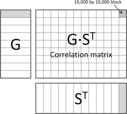
Matrix-eQTL strategies to reduce run time:

Required test statistic can be expressed in terms of the correlation between SNP and gene expression.
Use efficient matrix multiplications to compute the correlations.
Computing p-values is expensive, only do this for SNP/gene pairs that are sufficiently interesting.

Correcting for multiple testing

A genome-wide analysis requires estimating millions of effect sizes.
For an individual SNP/gene pair the p-value of the genotype coefficient may be a useful to gauge whether it is likely to be relevant.
Interpreting p-values becomes more difficult if millions of them have to be considered.

False discovery rate

Instead of considering each test individually try to control the number of tests that are incorrectly interpreted as indicating a true departure from the null hypothesis.
Adjust p-values such that the resulting value is an estimate of the proportion of false positives obtained at a given threshold.
Matrix-eQTL uses the Benjamini-Hochberg procedure.

Hands-on : Scaling it up

Data

Gene expression: /data/monocytes/expression/ifn_expression.tab.gz
Genotypes: /data/genotypes/genotypes.tab.gz
(downloaded earlier)

library(MatrixEQTL)
snps <- SlicedData$new()
snps$LoadFile("/data/genotypes/genotypes.tab.gz")
genes <- SlicedData$new()
genes$LoadFile("/data//monocytes/expression/ifn_expression.tab.gz")

Annotation data

Located in /data/monocytes/annotation/

snp_loc_hg19.tab: Genomic location of SNPs.
probe_loc_hg19.tab: Genomic location of gene expression probes.
probeAnnotations.tab: Further annotations for gene expression probes, including associated gene symbols.

probePos <- readr::read_tsv("/data/monocytes/annotation/probe_loc_hg19.tab")
snpPos <- readr::read_tsv("/data/monocytes/annotation/snp_loc_hg19.tab")
probeAnno <- readr::read_tsv("/data/monocytes/annotation/probeAnnotations.tab")

Running Matrix-eQTL

Use Matrix-eQTL to carry out a cis/trans eQTL analysis.

Use a 1MB window around probes as local association region
Use a p-value threshold of \(10^{-3}\) and \(10^{-5}\) for cis and trans associations respectively

Repeat the analysis with the first 10 PC included as covariates. How do results differ?

chr9.eQTL <- Matrix_eQTL_main(snps, genes,
        output_file_name="./ifn_chr9_eQTL.trans", 
        output_file_name.cis="./ifn_chr9_eQTL.cis", 
        pvOutputThreshold.cis=1e-3, snpspos=as.data.frame(snpPos), 
        genepos=as.data.frame(probePos))

pca <- prcomp(t(expr[-1]), center=TRUE, scale = TRUE)
pc <- pca$x

covar <- SlicedData$new()
covar$CreateFromMatrix(t(pc[,1:10]))

chr9.eQTL.pc10 <- Matrix_eQTL_main(snps, genes, cvrt=covar, 
        output_file_name="./ifn_chr9_eQTL.pc10.trans", 
        output_file_name.cis="./ifn_chr9_eQTL.pc10.cis", 
        pvOutputThreshold.cis=1e-3, snpspos=as.data.frame(snpPos), 
        genepos=as.data.frame(probePos))

Compare number of associations reported and take a look at p-values/FDR and effect sizes.
For trans associations in particular interesting results only start to appear after addition of PCs.

Interpreting results

Still just a pile of data

The initial analysis can produce a long list of SNP/gene associations.
Without further analysis these are not particularly helpful.
How can we identify particularly interesting results?
How can we assign biological meaning to the list of associations?

External data sources

A lot of genomic datasets and derived annotations are available.
Link SNPs to functional annotations using
Visualise SNPs in genomic context, e.g. using UCSC genome browser

Summary

We talked about

What eQTL are
How linear models can be used to find them
Complications that arise and possible approaches to deal with them
How to carry out large scale eQTL analyses
Some ideas of how to follow up on findings

We didn’t talk about

Details of data QC
The role of linkage disequilibrium in interpreting results
Comparison of eQTL between different conditions (tissues, treatments, …)
Other approaches to eQTL analysis (Bayesian, nonparametric)